Runge's phenomenon in Geogebra

Runge's phenomenon says roughly that a polynomial through equally spaced points over an interval will wobble a lot near the ends. Runge demonstrated this by fitting polynomials through equally spaced point in the interval \([-1,1]\) on the function \[ \frac{1}{1+25x^2} \] and this function is now known as "Runge's function".

It turns out that Geogebra can illustrate this extremely well.

Equally spaced vertices

Either open up your local version of Geogebra, or go to http://geogebra.org/graphing. In the boxes on the left, enter the following expressions in turn:

1. Start by entering Runge's function \[ f(x)=\frac{1}{1+25x^2} \] You should now either zoom in, or use the graph settings tool to display \(x\) between \(-1.5\) and \(1.5\).
2. Create a list of \(x\) values: \[ x1 = \frac{\{-5..5\}}{5} \]
3. Use those values to create a set of points on the curve: \[ p1 = (x1,f(x1)) \]
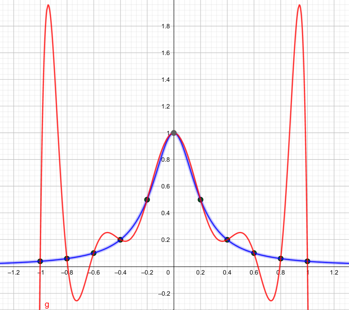
4. Now create an interpolating polynomial through them: \[ \mathsf{Polynomial}[p1(1)] \]

The resulting graph looks like this:

Chebyshev vertices

For the purpose of this post, we'll take the Chebyshev vertices to be those points in the graph whose \(x\) coordinates are given by

\[ x_k = \cos\left(\frac{k\pi}{10}\right) \] for \(k = 0,1,2,\ldots 10\). These values are more clustered at the ends of the interval.

In Geogebra:

1. As before, enter the \(x\) values first: \[ x2 = \cos(\frac{\{0..10\}\cdot\pi}{10}) \]
2. Then turn them into a sequence of points on the curve \[ p2 = (x2,f(x2)) \]
3. Finally create the polynomial through them: \(\mathsf{Polynomial}(p2(1))\).

And this graph looks like this:

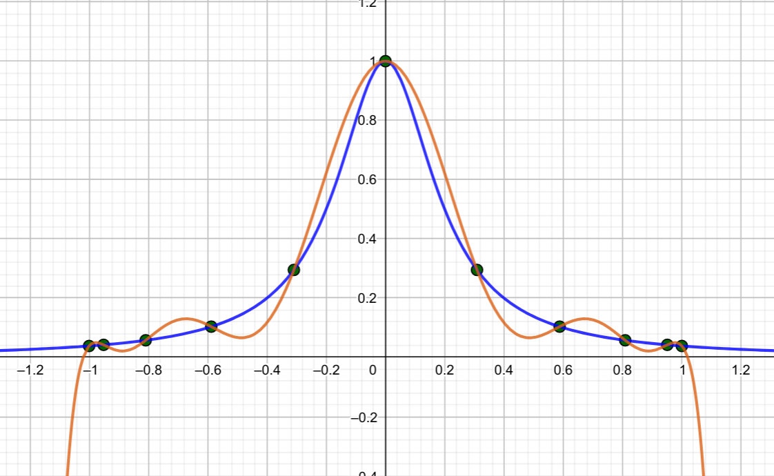
You'll notice how better the second polynomial hugs the curve. The issue is even more pronounced with 21 points, either separated by \(0.1\), or with \(x\) values given by the cosine function again. All we need do is to change the definitions of the \(x\) value sequences \(x1\) and \(x2\) to:

\[ \eqalign{ x1 &= \frac{\{-10..10\}}{10}\\ x2 &= \cos(\frac{\{0..20\}\pi}{20}) } \]

In fact, you can create a slider \(1\le N \le 20\), say, and then define

\[ \eqalign{ x1 &= \frac{\{-N..N\}}{N}\\ x2 &= \cos(\frac{\{0..2N\}\pi}{2N}) } \]

and then see how as \(N\) increases, the "Chebyshev" interpolant fits the curve better than the equally spaced interpolant. For \(N=20\), the turning points of the equally spaced polynomial have \(y\) values as high as \(59.78\).

Integration

Using equally spaced values to create an interpolating polynomial and then integrating that polynomial is Newton-Cotes integration. Runge's phenomenon shows why it is better to partition the interval into small sub-intervals and apply a low-order rule to each one. For example, with 20 points on the curve, we would be better applying Simpson's rule to each pair of two sub-intervals, and adding the result. Using a 21-point polynomial is equivalent to a Newton-Cotes rule of order 20, which is far too inaccurate to use.

With our curve \(f(x)\), and our equal-spaced polynomial \(g(x)\), the integrals are

\[ \eqalign{ \int^1_{-1}\frac{1}{1+25x^2}\,dx&=\frac{2}{5}\arctan(5)\approx 0.5493603067780064\\ \int^1_{-1}g(x)\,dx&\approx -5.369910417304622 } \]

However, using the polynomial through the Chebyshev nodes:

\[ \int^1_{-1}h(x)\approx 0.5498082303389538. \]

The absolute errors between the integral values and the exact values are thus (approximately) \(5.92\) and \(0.00045\) respectively.

Integrating an interpolating polynomial through Chebyshev nodes is one way of implementing Clenshaw-Curtis quadrature.

Note that using Simpson's rule on our 21 points produces a value of 0.5485816035037206, which has absolute error of about \(0.0012\).