Image dithering (2): error diffusion

A totally different approach to dithering is error diffusion. Here, the image is scanned pixel by pixel. Each pixel is thresholded t0 1 or 0 depending on whether the pixel value is greater than 0.5 or not, and the error - the difference between the pixel value and its threshold - is diffuse across neighbouring pixels.

The first method was developed by Floyd and Steinberg, who proposed the following diffusion:

\[\frac{1}{16}\begin{bmatrix} &*&7\\ 3&5&1 \end{bmatrix}\]

What this means is that if the current pixel's value is \(m_{ij}\), it will be thresholded to 1 or 0 depending on whether its value is greater than 0.5 or not. We set

\[t_{ij}=\left\{\begin{array}{ll}1&\mbox{if $m_{ij}>0.5$}\\ 0&\mbox{otherwise}\end{array}\right.\]

Alternatively,

\[t_{ij} = m_{ij}>0.5\]

assuming that the right hand expression returns 1 for true, 0 for false. Then the error is

\[e_{ij}=m_{ij}-t_{ij}\].

The surrounding pixels are then updated by fractions of this error:

\[\begin{align*} m_{i,j+1}&=m_{i,j+1}+\frac{7}{16}e_{ij}\\ m_{i+1,j-1}&=m_{i+1,j-1}+\frac{3}{16}e_{ij}\\ m_{i+1,j}&=m_{i+1,j}+\frac{5}{16}e_{ij}\\ m_{i+1,j+1}&=m_{i+1,j+1}+\frac{1}{16}e_{ij} \end{align*}\]

There is a Julia package for computing error diffusion called DitherPunk, but in fact the basic logic can be easily managed:

 1Julia> r,c = size(img)
 2Julia> out = Float64.(image)
 3Julia> fs = [0 0 7;3 5 1]/16
 4Julia> for i = :r-1
 5	   for j = 2:c-1
 6	       old = out[i,j]
 7	       new = round(old)
 8	       out[i,j] = new
 9	       error = old - new
10	       out[i:i+1,j-1:j+1] += error * fs
11	   end
12       end

To ensure that the final image is the same size as the original, we can just take the central, changed pixels, and pad them by replication:

1Julia> padding = Pad(:replicate, (0,1),(1,1))
2Julia> out = paddarray(out[1:r-1, c-1:c+1], padding)
3Julia> out = Gray.(abs.(out))

Here's the result applied to the bridge image from before, again with the original image for comparison:

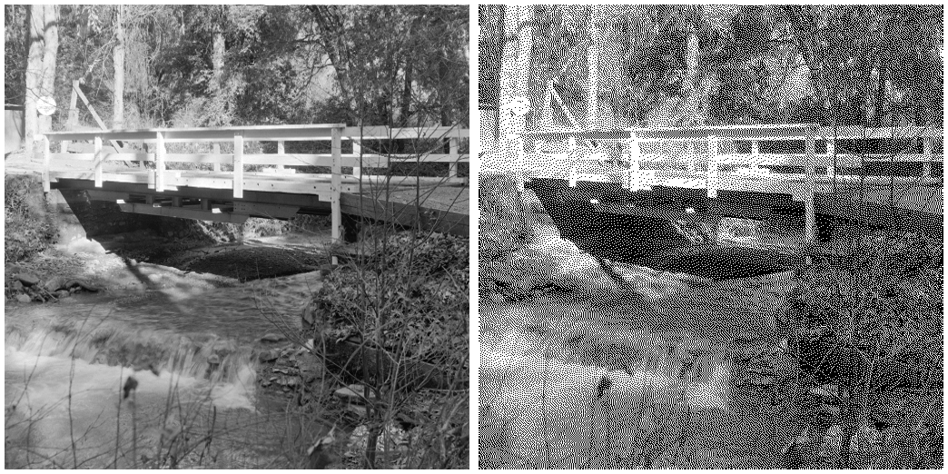
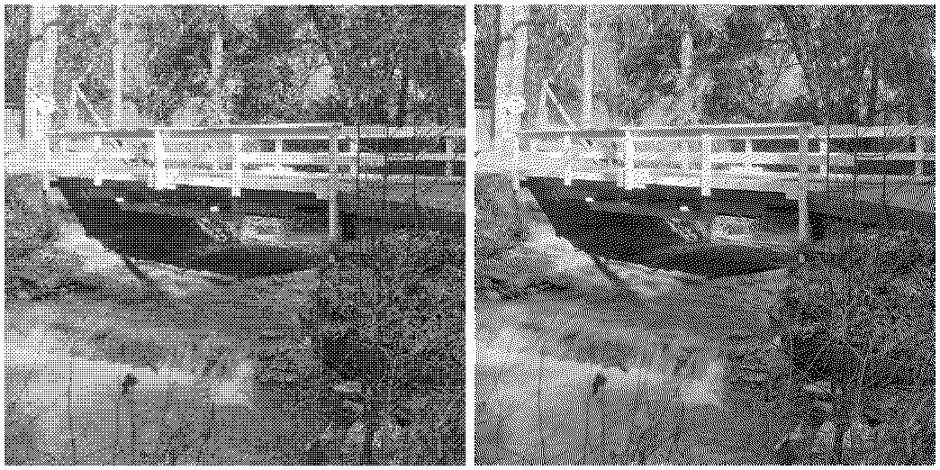
If you compare this dithered image with the halftoned image from the last blog post, you'll notice some slight cross-hatching in the halftoned image; this is an artefact of the repetition of the B4 Bayer matrix. Such an artefact doesn't exist in the error-diffused image. To make that comparison easier, here they both are, with the half-tone image on the left, and the image with error diffusion on the right:

Error diffusion has the added advantage of being able to produce an output of more than two levels; this allows the number of colours in an image to be reduced while at the same time reducing the degradation of the image.

If we want \(k\) output grey values, from 0 to \(k-1\), all we do is change the definition of new in the loop given above to

1new = round(old * (k-1)) / (k-1)

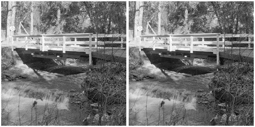
Here, for example, is the same image with 4 and with 8 grey levels:

The above process for dithering can easily be adjusted for any other dither matrices, of which there are many, for example:

Jarvice-Judice-Ninke:

\[\frac{1}{48}\begin{bmatrix} 0& 0& *& 7& 5\\3& 5& 7& 5& 3\\1& 3& 5& 3& 1 \end{bmatrix}\]

Stucki:

\[\frac{1}{42}\begin{bmatrix} 0& 0& *& 8& 4\\2& 4& 8& 4& 2\\1& 2& 4& 2& 1 \end{bmatrix}\]

Atkinson:

\[\frac{1}{8}\begin{bmatrix} 0& *& 1& 1\\1& 1& 1& 0\\0& 1& 0& 0 \end{bmatrix}\]

Burke:

\[\frac{1}{32}\begin{bmatrix} 0& 0& *& 8& 4\\2& 4& 8& 4& 2 \end{bmatrix}\]

Sierra:

\[\frac{1}{32}\begin{bmatrix} 0& 0& *& 5& 3\\2& 4& 5& 4& 2\\0& 2& 3& 2& 0 \end{bmatrix}\]

Two row Sierra:

\[\frac{1}{16}\begin{bmatrix} 0& 0& *& 4& 3\\1& 2& 3& 2& 1 \end{bmatrix}\]

Sierra Lite

\[\frac{1}{4}\begin{bmatrix} 0& *& 2\\ 1& 1& 0 \end{bmatrix}\]

Note that the DitherPunk package is named after a very nice blog post discussing dithering. This post makes reference to another post which discusses dithering in the context of the game Return of the Obra Dinn. This game is set in the year 1807, and to obtain a sort of "antique" look, its developer used dithering techniques extensively to render all scenes using "1-bit graphics". A glimpse at its trailer will show you how well this has been done. (Note: I haven't played the game; I'm not a game player. But as with all games there are plenty of videos - some many hours long - about the game and playing it.)

Colour images

Dithering of colour images is very simple: simple dither each of the red, green and blue colour planes, then put them all back together. Assuming the above process for grey level dithering has been encapsulated in a function called dither, we can write:

1function cdither(image;nlevels = 2)
2    image_rgb = channelview(image)
3    rd = dither(image_rgb[1,:,:],nlevels)
4    gd = dither(image_rgb[2,:,:],nlevels)
5    bd = dither(image_rgb[3,:,:],nlevels)
6    image_d = colorview(RGB, rd,gd,bd)
7    return(image_d)
8end

Here, for example, are the results of dithering at two and four levels of the "lighthouse" image from the test images database:

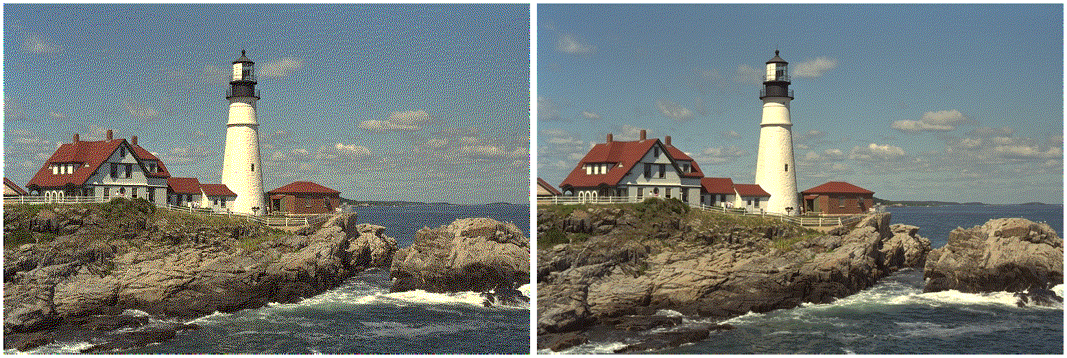
The first image shows some artefacts as noise, but is still remarkably clear; the second image is surprisingly good. If the three images (original, two-level dither, four-level dither) are saved into variables img, img_d2, img_d4, then:

1Julia> [length(unique(x) for x in [img,img_d2,img_d4]]'
2
31×3 adjoint(::Vector{Int64}) with eltype Int64:
4 29317  8  34

So the second image, clear as it is, uses only 34 distinct colours as opposed to the nearly 30000 of the original image.