Mapping voting gains between elections
So this goes back quite some time to the recent Australian Federal election on May 18. In my own electorate (known formally as a “Division”) of Cooper, the Greens, who until recently had been showing signs of winning the seat, were pretty well trounced by Labor.
Some background asides
First, “Labor” as in “Australian Labor Party” is spelled the American way; that is, without a “u”, even though “labour” meaning work, is so spelled in Australian English. This is because much of Australia’s pre-federal political history has a large American influence; indeed one of the loudest political voices in the 19th century was King O’Malley who was born in 1858 in Kansas, and didn’t come to Australia until he was about 30. He was responsible, amongst other things, for selecting the site for Canberra (the nation’s capital) and in selecting Walter Burley Griffin as its architect. As well, the Australian Constitution shows a large American influence; the constitutions of both countries bear a remarkably close resemblance, and Australia’s parliament is modelled on that of the United States Congress.
Second, my electorate was formerly known as “Batman” after John Batman, the supposed founder of Melbourne. However, Batman was known in his lifetime as a contemptible figure, and the historical record well bears out the description of him as “the vilest man I have ever known”. He was responsible for the slaughter of indigenous peoples, and his so called “treaty” with the people of the Kulin Nation in exchange for land on what would would become Melbourne is considered invalid. In respect for the local peoples (“who have never ceded sovereignty”), the electorate was renamed last year in honour of William Cooper, a Yorta Yorta elder, a tireless activist for Aboriginal rights, and the only individual in the world to lodge a formal protest to a German embassy on the occasion of Kristallnacht.
Back to mapping
All I wanted to do was to map the size of Labor’s gains (over the Greens) between the last election in 2016 and this one, at each polling booth in the electorate. For this I used the following Python packages: matplotlib, pandas, geopandas, numpy, cartopy. The nice thing about Python, for me at least, is the ease of prototyping, and the availability of packages for just about everything. Indeed, for an amateur programmer like myself, one of the biggest difficulties is finding the right package for the job. There’s a score or more for GIS alone.
All information about the election can be downloaded from the Australian Electorial Commission tallyroom. And the GIS information can be obtained also from the AES. The Victorian shapefile needs to be unzipped before using.
Then the map set-up looks like this:
shp = gpd.read_file('VicMaps/E_AUGFN3_region.shp')
cooper = shp.loc[shp['Elect_div']=='Cooper']
bounds = cooper.geometry.bounds
bg = bounds.values[0]  # latitude, longitude of extent of region
pad = 0.01             # padding for display
extent = [bg[0]-pad,bg[2]+pad,bg[1]-pad,bg[3]+pad]
The idea of the padding is simply to ensure that the map, once displayed, extends beyond the area of the electorate. The units are degrees of latitude and longitude. In Melbourne, at about 37.8 degrees south, 0.01 degrees latitude corresponds to about 1.11km, and 0.01 degrees longitude corresponds to about 0.88km.
Now we need to determine the percentage of votes to Labor (on a two-party preferred computation) which again involves reading material from the AEC site. I downloaded it first, but it could also be read directly from the site into pandas.
# Get all votes by polling booths in Cooper for 2019
b19 = pd.read_csv('Elections/TCPByCandidateByPollingPlaceVIC-2019.csv')  # b19 = booths, 2019
v19 = b19.loc[b19.DivisionNm=='Cooper'] # v19 = Cooper Booths, 2019
v19 = v19[['PollingPlace','PartyAb','OrdinaryVotes']]
v19r = v19.loc[v19.PartyAb=='GRN']
v19k = v19.loc[v19.PartyAb=='ALP']
v19c = v19r.merge(v19k,left_on='PollingPlace',right_on='PollingPlace')  # Complete votes
v19c['Percent_x'] = (v19c['OrdinaryVotes_x']*100/(v19c['OrdinaryVotes_x']+v19c['OrdinaryVotes_y'])).round(2)
v19c['Percent_y'] = (v19c['OrdinaryVotes_y']*100/(v19c['OrdinaryVotes_x']+v19c['OrdinaryVotes_y'])).round(2)
v19c = v19c.dropna()
# note: suffix -x is GRN; suffix _y is ALP
The next step is to determine the positions of all polling places. For simplification, I’m only interested in places used in both this most recent election, and the previous federal election in 2016:
v16 = pd.read_csv('Elections/Batman2016_TCP.csv')
v_both = v16.merge(v19c,right_on='PollingPlace',left_on='Booth')
c19 = pd.read_csv('Elections/Cooper_PollingPlaces.csv')
c19 = c19.drop(44).reset_index()  # Drop Special Hospital, which has index 44
v_all=v_both.merge(c19,left_on='PollingPlace',right_on='PollingPlaceNm')
lats = np.array(v_all['Latitude'])
longs = np.array(v_all['Longitude'])
booths = np.array(v_all['PollingPlaceNm'])
diffs = np.array(v_all['Percent_y']-v_all['ALP percent']) # change in ALP percentage
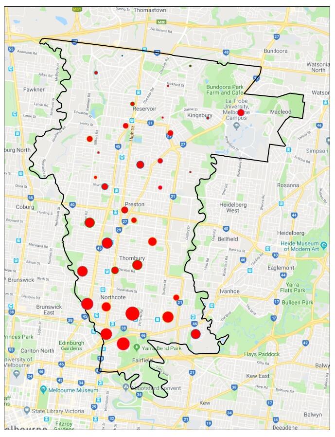
Having now got the boundary of the electorate, the positions of each polling booth, the percentage change in votes for Labor, the map can now be created and displayed:
fig = plt.figure(figsize = (16,16))
tiler = GoogleTiles()
ax = plt.axes(projection=tiler.crs)
ax.set_extent(extent)
ax.add_image(tiler, 13, interpolation='hanning')
ax.add_geometries(cooper.geometry,crs=ccrs.PlateCarree(),facecolor='none',edgecolor='k',linewidth=2)
for i in range(34):
    if diffs[i]>0:
        ax.plot(longs[i],lats[i],marker='o',markersize=diffs[i],markerfacecolor='r',transform=ccrs.Geodetic())
    else:
        ax.plot(longs[i],lats[i],marker='o',markersize=-diffs[i],markerfacecolor='g',transform=ccrs.Geodetic())
plt.show()
I found by trial and error that Hanning interpolation seemed to give the best results.
So this image shows not the size of Labor’s vote, but the size of Labor’s gain since the previous election. The larger gains are in the southern part of the electorate: the northern part has always been more Labor friendly, and so the gains were smaller there.