Post-election swings
So the Australian federal election of 2022 is over as far as the public is concerned; all votes have been cast and now it's a matter of waiting while the Australian Electoral Commission tallies the numbers, sorts all the preferences, and arrives at a result. Because of the complications of the voting system, and of all the checks and balances within it, a final complete result may not be known for some days or even weeks. What is known, though, is that the sitting government has been ousted, and that the Australian Labor Party (ALP) will lead the new government. Whether the ALP amasses enough wins for it to govern with a complete majority is not known; they may have a "minority government" in coalition with either independent candidates or the Greens.
In Australia, there are 151 federal electorates or "Divisions"; each one corresponds to seat in the House of Representatives; the Lower House of the Federal government. The winner of an election is whichever party or coalition wins the majority of seats; the Prime Minister is simply the leader of the major party in that coalition. Australians thus have no say whatsoever in the Prime Minister; that is entirely a party matter, which is why Prime Ministers have sometimes been replaced in the middle of a term.
My concern is the neighbouring electorates of Cooper and Wills. Both are very similar both geographically and politically; both are Labor strongholds, in each of which the Greens have made considerable inroads. Indeed Cooper (called Batman until a few years ago) used to be one of the safest Labor seats in the country; it has now become far less so, and in each election the battle is now between Labor and the Greens. Both are urban seats, in Melbourne; in each of them the southern portion is more gentrified, diverse, and left-leaning, and the Northern part is more solidly working-class, and Labor-leaning. In each of them the dividing line is [Bell St](https://en.wikipedia.org/wiki/State_(Bell/Springvale)_Highway), known as the "tofu curtain". (Also as the "Latte Line" or the "Hipster-Proof Fence".)
Thus Greens campaigning consists of letting the southerners know they haven't been forgotten, and attempting to reach out to the northerners. This is mainly done with door-knocking by volunteers, and there is never enough time, or enough volunteers, to reach every household.
Anyway, here are some maps showing the Greens/Labor result at each polling booth. The size of the circle represents the ratio of votes: red for a Labor majority; green for a Greens majority. And the popup tooltip gives the name of the polling booth, and the swing either to Labor or to the Greens.
I couldn't decide the best way of displaying the swings, so in the end I just displayed the swing to Labor in all booths with a Labor majority, even if that swing was sometimes negative. And similarly for the Greens. Note that a large swing may correspond to a relatively small number of votes being cast.
If you get the shape into a state from which you can't get the stair affect working, click on the little circular arrows in the bottom left, which will reset the object to its initial orientation.
Impossible box
This was just a matter of creating the edges, finding a nice view, and using some trial and error to slice through the front most beams so that it seemed that hhe read beams were at the front.
Here is another widget, again you may have to wait for it to load.
Voting power (4): Speeding up the computation
Introduction and recapitulation
Recall from previous posts that we have considered two power indices for computing the power of a voter in a weighted system; that is, the ability of a voter to influence the outcome of a vote. Such systems occur when the voting body is made up of a number of "blocs": these may be political parties, countries, states, or any other groupings of people, and it is assumed that within every bloc all members will vote the same way. Indeed, in some legislatures, voting according to "the party line" is a requirement of membership.
Examples include the American Electoral College, in which the "voters" are the states; the Australian Senate, the European Union, the International Monetary Fund, and many others.
Given a set \(N=\{1,2,\ldots,n\}\) of voters and their weights \(w_i\), and a quota \(q\) required to pass any motion, we have represented this as
\[ [q;w_1,w_2,\ldots,w_n] \]
and we define a winning coalition as any subset \(S\subset N\) of voters for which
\[ \sum_{i\in S}w_i\ge q. \]
It is convenient to define a characteristic function \(v\) on all subsets of \(N\) so that \(v(S)=1\) if \(S\) is a winning coalition, and 0 otherwise. Given a winning coalition \(S\), a voter \(i\in S\) is necessary if \(v(S)-v(S-\{i\})=1\).
For any voter \(i\), the number of winning coalitions for which that voter is necessary is
\[ \beta_i = \sum_S\left(v(S)-v(S-\{i\})\right) \]
where the sum is taken over all winning coalitions. Then the Banzhaf power index is this value normalized so that the sum of all indices is unity:
\[ B_i=\frac{\beta_i}{\sum_{i=1}^n \beta_i}. \]
The Shapley-Shubik power index is defined by considering all permutations \(p\) of \(N\). Taken cumulative sums from the left, a voter \(p_k\) is pivotal if this is the first voter for which te cumulative sum is at least \(q\). For each voter \(i\), let \(\sigma_i\) be the number of permutations for which \(i\) is pivotal. Then
\[ S_i=\frac{1}{n!}\sigma_i \]
which ensures that the sum of all indices is unity.
Although these two indices seem very different, there is in fact a deep connection. Consider any permutation \(p\) and suppose that \(i=p_k\) is the pivotal voter, This voter will also be pivotal in all permutations for which \(i=p_k\) and the values to the right and left of \(i\) stay there: there will be \((k-1)!(n-k)!\) such permutations. However, we can consider the values up to and including \(i=p_k\) as a winning coalition for which \(i\) is necessary, which means we can write
\[ S_i=\sum_S\frac{(n-k)!(k-1)!}{n!}\left(v(S)-v(S-\{i\})\right) \]
which can be compared to the Banzhaf index above as being similar and with a different weighting function. Note that the above expression can be written as
\[ S_i=\sum_S\left(k{\dbinom n k}\right)^{-1}\left(v(S)-v(S-\{i\})\right) \]
which uses smaller numbers. For example, if \(n=50\) then \(n!\approx 3.0149\times 10^{64}\) but the largest binomial value is only approximately \(1.264\times 10^{14}\).
Computing with polynomials
We have also seen that if we define
\[ f_i(x) = \prod_{m\ne i}(1+x^{w_m}) \]
then
\[ \beta_i = \sum_{j=q-w_i}^{q-1}a_j \]
where \(a_j\) is the coefficient of \(x_j\) in \(f_i(x)\).
Similarly, if
\[ f_i(x,y) = \prod_{m\ne i}(1+yx^{w_m}) \]
then
\[ S_i=\sum_{k=0}^{n-1}\frac{k!(n-1-k)!}{n!}\sum_{j=q-w_i}^{q-1}c_{jk} \]
where \(c_{jk}\) is the coefficient of \(x^jy^k\) in the expansion of \(f_i(x,y)\).
In a previous post we have shown how to implement these in Python, using the Sympy library. However, Python can be slow, and using Cython is not trivial. We thus here show how to use Julia and its Polynomials package.
Using Julia for speed
The Banzhaf power indices can be computed almost directly from the definition:
using Polynomials

function px(n)
    return(Polynomial([0,1])^n)
end

function banzhaf(q,w)
    n = length(w)
    inds = vec(zeros(Int64,1,n))
    for i in 1:n
	p = Polynomial([1])
	for j in 1:i-1
	    p = p * px(v[j])
	end
	for j in i+1:n
	    p = p*px(v[j])
	end
	inds[i] = sum(coeffs(p)[k] for k in q-w[i]+1:q)
    end
    return(inds)
end
This will actually return the vector of \(\beta_i\) values which can then be easily normalized.
The function px is a "helper function" that simply returns the polynomial \(x^n\).
For the Shapley-Shubik indices, the situation is a bit trickier. There are indeed some Julia libraries for multivariate polynomials, but they seem (at the time of writing) to be not fully functional. However, consider the polynomials
\[ f_i(x,y)=\prod_{m\ne i}(1+yx^{w_m}) \]
from above. We can consider this as a polynomial of degree \(n-1\) in \(y\), whose coefficients are polynomials in \(x\). So if
\[ f_i(x,y) = 1 + p_1(x)y + p_2(x)y^2 +\cdots + p_{n-1}(x)y^{n-1} \]
then \(f_i(x,y)\) can be represented as a vector of polynomials
\[ [1,p_1(x),p_2(x),\ldots,p_{n-1}(x)]. \]
With this representation, we need to perform a multiplication by \(1+yx^p\) and also determine coefficients.
Multiplication is easy, noting at once that \(1+yx^p\) is linear in \(y\), and so we use the expansion of the product
\[ (1+ay)(1 + b_1y + b_2y^2 + \cdots + b_{n-1}y^{n-1}) \]
to
\[ 1 + (a+b_1)y + (ab_1+b_2)y^2 + \cdots + (ab_{n-2}+b_{n-1})y^{n-1} + ab_{n-1}y^n. \]
This can be readily programmed as:
function mulp1(n,p)
    p0 = Polynonial(0)
    px = Polynomial([0,1])
    c1 = cat(p,p0,dims=1)
    c2 = cat([p0,p,dims=1)
    return(c1 + px^n .* c2)
end
The first two lines aren't really necessary, but they do make the procedure easier to read.
And we need a little program for extracting coefficients, with a result of zero
if the power is greater than the degree of the polynomial (Julia's coeff
function simply produces a list of all the coefficients in the polynomial.)
function one_coeff(p,n)
    d = degree(p)
    pc = coeffs(p)
    if n <= d
	return(pc[n+1])
    else
	return(0)
    end
end
Now we can put all of this together in a function very similar to the Python function for computing the Shapley-Shubik indices with polynomials:
function shapley(q,w)
    n = length(w)
    inds = vec(zeros(Float64,1,n))
    for i in 1:n
	p = Polynomial(1)
	for j in 1:i-1
	    p = mulp1(w[j],p)
	end
	for j in i+1:n
	    p = mulp1(w[j],p)
	end
	B = vec(zeros(Float64,1,n))
	for j in 1:n
	    B[j] = sum(one_coeff(p[j],k) for k in q-w[i]:q-1)
	end
	inds[i] = sum(B[j+1]/binomial(n,j)/(n-j) for j in 0:n-1)
    end
    return(inds)
end
And a quick test (with timing) of the powers of the states in the Electoral
College; here ecv is the number of electors of all the states, in
alphabetical order (the first states are Alabama, Alaska, Arizona, and the last
states are West Virginia, Wisconsin, Washington):
ecv = [9, 3, 11, 6, 55, 9, 7, 3, 3, 29, 16, 4, 4, 20, 11, 6, 6, 8, 8, 4, 10, 11, 16, 10, 6,
10, 3, 5, 6, 4, 14, 5, 29, 15, 3, 18, 7, 7, 20, 4, 9, 3, 11, 38, 6, 3, 13, 12, 5, 10, 3]
@time(s = shapley(270,ecv));
0.722626 seconds (605.50 k allocations: 713.619 MiB, 7.95% gc time)
This is running on a Lenovo X1 Carbon, 3rd generation, using Julia 1.5.3. The operating system is a very recently upgraded version of Arch Linux, and currently using kernel 5.10.3.
Voting power (3): The American swing states
As we all know, American Presidential elections are done with a two-stage process: first the public votes, and then the Electoral College votes. It is the Electoral College that actually votes for the President; but they vote (in their respective states) in accordance with the plurality determined by the public vote. This unusual system was devised by the Founding Fathers as a compromise between mob rule and autocracy, of which both they were determined to guard against. The Electoral College is not now an independent body: in all states but two all electoral college votes are given to the winner in that state. This means that the Electoral College may "amplify" the public vote; or it may return a vote which differs from the public vote, in that a candidate may receive a majority of public votes, and yet still lose the Electoral College vote. This means that there are periodic calls for the Electoral College to be disbanded, but in reality that seems unlikely. And in fact as far back as 1834 the then President, Andrew Jackson, was demanding its disbanding: a President, according to Jackson, should be a "man of the people" and hence elected by the people, rather than by an elite "College". This is one of the few instances where Jackson didn't get his way.
The initial idea of the Electoral College was that voters in their respective states would vote for Electors who would best represent their interests in a Presidential vote: these Electors were supposed to be wise and understanding men who could be relied on to vote in a principled manner. Article ii, Section 1 of the USA Constitution describes how this was to be done. When it became clear that electors were not in fact acting impartially, but only at the behest of the voters, some of the Founding Fathers were horrified. And like so many political institutions the world over, the Electoral College does not now live up to its original expectations, but is also too entrenched in the political process to be removed.
The purpose of this post is to determine the voting power of the "swing states", in which most of a Presidential campaign is conducted. It has been estimated that something like 75% of Americans are ignored in a campaign; this might be true, but that's just plain politics. For example California (with 55 Electoral College cotes) is so likely to return a Democrat candidate that it may be considered a "safe state" (at least, for the Democrats); it would be a waste of time for a candidate to spend too much time there. Instead, a candidate should stump in Florida, for example, which is considered a swing state, and may go either way: we have seen how close votes in Florida can be.
For discussion about measuring voting power using power indices check out the previous two blog posts.
The American Electoral College
According to the excellent site 270 to win and their very useful election histories, we can determine which states have voted "the same" for any election post 1964. Taking 2000 as a reasonable starting point, we have the following results. Some states have voted the same in every election from 2000 onwards; others have not.
| Safe Democrat | Safe Republican | Swing | |||
|---|---|---|---|---|---|
| California | 55 | Alabama | 9 | Colorado | 9 |
| Connecticut | 7 | Alaska | 3 | Florida | 29 |
| Delaware | 3 | Arizona | 11 | Idaho | 4 |
| DC | 3 | Arkansas | 6 | Indiana | 11 |
| Hawaii | 4 | Georgia | 16 | Iowa | 6 |
| Illinois | 20 | Kansas | 6 | Michigan | 16 |
| Maine | 3 | Kentucky | 8 | Nevada | 6 |
| Maryland | 10 | Louisiana | 8 | New Hampshire | 4 |
| Massachusetts | 11 | Mississippi | 6 | New Mexico | 5 |
| Minnesota | 10 | Missouri | 10 | North Carolina | 15 |
| New Jersey | 14 | Montana | 3 | Ohio | 18 |
| New York | 29 | Nebraska | 4 | Pennsylvania | 20 |
| Oregon | 7 | North Dakota | 3 | Virginia | 13 |
| Rhode Island | 4 | Oklahoma | 7 | Wisconsin | 10 |
| Vermont | 3 | South Carolina | 9 | Maine CD 2 | 1 |
| Washington | 12 | South Dakota | 3 | Nebraska CD 2 | 1 |
| Tennessee | 11 | ||||
| Texas | 38 | ||||
| Utah | 6 | ||||
| West Virginia | 5 | ||||
| Wyoming | 3 | ||||
| 195 | 175 | 168 |
From the table, we see that since 2000, we can count on 195 "safe" Electoral College votes for the Democrats, and 175 "safe" Electoral College votes for the Republicans. Thus of the 168 undecided votes, for a Democrat win the party must obtain at least 75 votes, and for a Republican win, the party needs to amass 95 votes.
Note that according to the site, of the votes in Maine and Nebraska, all but one are considered safe - remember that these are the only two states to apportion votes by Congressional district. Of Maine's 4 Electoral College votes, 3 are safe Democrat and one is a swing vote; for Nebraska, 4 of its votes are safe Republican, and 1 is a swing vote.
All this means is that a Democrat candidate should be campaigning considering the power given by
\[ [75; 9,29,4,11,6,16,6,4,5,15,18,20,13,10,1,1] \]
and a Republican candidate will be working with
\[ [95; 9,29,4,11,6,16,6,4,5,15,18,20,13,10,1,1] \]
A Democrat campaign
So let's imagine a Democrat candidate who wishes to maximize the efforts of the campaign by concentrating more on states with the greatest power to influence the election.
In [1]: q = 75; w = [9,29,4,11,6,16,6,4,5,15,18,20,13,10,1,1]

In [2]: b = banzhaf(q,w); bn = [sy.Float(x/sum(b)) for x in b]; [sy.N(x,4) for x
in bn]
Out[2]: [0.05192, 0.1867, 0.02271, 0.06426, 0.03478, 0.09467, 0.03478, 0.02271,
0.02870, 0.08801, 0.1060, 0.1196, 0.07515, 0.05800, 0.005994, 0.005994]

In [3]: s = shapley(q,w); [sy.N(x/sum(s),4) for x in s]
out[3]: [0.05102, 0.1902, 0.02188, 0.06375, 0.03367, 0.09531, 0.03367, 0.02188,
0.02770, 0.08833, 0.1073, 0.1217, 0.07506, 0.05723, 0.005662, 0.005662]
The values are not the same, but they are in fact quite close, and in this case they are comparable to the numbers of Electoral votes in each state. To compare values, it will be most efficient to set up a Dataframe using Python's data analysis library pandas. We shall also convert the Banzhaf and Shapley-Shubik values from sympy floats int ordinary python floats.
In [4]: import pandas as pd
In [5]: bf = [float(x) for x in bn]
In [6]: sf = [float(x) for x in s]

In [5]: d = {"States":states, "EC Votes":ec_votes, "Banzhaf indices":bf, "Shapley-Shubik indices:sf}

In [6]: swings = pd.DataFrame(d)

In [7]: swings.sort_values(by = "EC Votes", ascending = False)
In [8]: ssings.sort_values(by = "Banzhaf indices", ascending = False)
In [9]: swings.sort_values(by = "Shapley-Shubik indices", ascending = False)
We won't show the results of the last three expressions, but they all give rise to the same ordering.
We can still get some information by not looking so much at the values of the power indices, but their relative values to the number of Electoral votes. To do this we need a new column which normalizes the Electoral votes so that their sum is unity:
In [10]: swings["Normalized EC Votes"] = swings["EC Votes"]/168.0
In [11]: swings["Ratio B to N"] = swings["Banzhaf indices"]/swings["Normalized EC Votes"]
In [12]: swings["Ratio S to N"] = swings_d["Shapley-Shubik indices"]/swings["Normalized EC Votes"]
In [13]: swings.sort_values(by = "EC Votes", ascending = False)
The following table shows the result.
| States | EC Votes | Banzhaf indices | Shapley-Shubik indices | EC Votes Normalized | Ratio B to N | Ratio S to N |
|---|---|---|---|---|---|---|
| Florida | 29 | 0.186702 | 0.190164 | 0.172619 | 1.081585 | 1.101640 |
| Pennsylvania | 20 | 0.119575 | 0.121732 | 0.119048 | 1.004430 | 1.022552 |
| Ohio | 18 | 0.106034 | 0.107289 | 0.107143 | 0.989655 | 1.001360 |
| Michigan | 16 | 0.094671 | 0.095309 | 0.095238 | 0.994049 | 1.000743 |
| North Carolina | 15 | 0.088014 | 0.088330 | 0.089286 | 0.985754 | 0.989293 |
| Virginia | 13 | 0.075149 | 0.075057 | 0.077381 | 0.971155 | 0.969966 |
| Indiana | 11 | 0.064261 | 0.063752 | 0.065476 | 0.981447 | 0.973660 |
| Wisconsin | 10 | 0.058004 | 0.057227 | 0.059524 | 0.974471 | 0.961422 |
| Colorado | 9 | 0.051922 | 0.051017 | 0.053571 | 0.969215 | 0.952318 |
| Iowa | 6 | 0.034777 | 0.033670 | 0.035714 | 0.973770 | 0.942774 |
| Nevada | 6 | 0.034777 | 0.033670 | 0.035714 | 0.973770 | 0.942774 |
| New Mexico | 5 | 0.028695 | 0.027704 | 0.029762 | 0.964169 | 0.930862 |
| Idaho | 4 | 0.022714 | 0.021877 | 0.023810 | 0.953972 | 0.918823 |
| New Hampshire | 4 | 0.022714 | 0.021877 | 0.023810 | 0.953972 | 0.918823 |
| Maine CD 2 | 1 | 0.005994 | 0.005662 | 0.005952 | 1.007058 | 0.951282 |
| Nebraska CD 2 | 1 | 0.005994 | 0.005662 | 0.005952 | 1.007058 | 0.951282 |
We can thus infer that a Democrat candidate should indeed campaign most vigorously in the states with the largest number of Electoral votes. This might seem to be obvious, but as we have shown in previous posts, there is not always a correlation between voting weight and voting power, and that a voter with a low weight might end up having considerable power.
A Republican candidate
Going through all of the above, but with a quota of 95, produces in the end the following:
| States | EC Votes | Banzhaf indices | Shapley-Shubik indices | EC Votes Normalized | Ratio B to N | Ratio S to N |
|---|---|---|---|---|---|---|
| Florida | 29 | 0.186024 | 0.190086 | 0.172619 | 1.077658 | 1.101190 |
| Pennsylvania | 20 | 0.119789 | 0.121871 | 0.119048 | 1.006230 | 1.023718 |
| Ohio | 18 | 0.106258 | 0.107258 | 0.107143 | 0.991741 | 1.001075 |
| Michigan | 16 | 0.094453 | 0.095156 | 0.095238 | 0.991756 | 0.999140 |
| North Carolina | 15 | 0.088106 | 0.088410 | 0.089286 | 0.986789 | 0.990194 |
| Virginia | 13 | 0.075362 | 0.074940 | 0.077381 | 0.973906 | 0.968460 |
| Indiana | 11 | 0.064064 | 0.063568 | 0.065476 | 0.978439 | 0.970862 |
| Wisconsin | 10 | 0.058073 | 0.057394 | 0.059524 | 0.975628 | 0.964219 |
| Colorado | 9 | 0.052133 | 0.051209 | 0.053571 | 0.973140 | 0.955892 |
| Iowa | 6 | 0.034692 | 0.033612 | 0.035714 | 0.971363 | 0.941142 |
| Nevada | 6 | 0.034692 | 0.033612 | 0.035714 | 0.971363 | 0.941142 |
| New Mexico | 5 | 0.028776 | 0.027715 | 0.029762 | 0.966885 | 0.931235 |
| Idaho | 4 | 0.022912 | 0.021963 | 0.023810 | 0.962300 | 0.922436 |
| New Hampshire | 4 | 0.022912 | 0.021963 | 0.023810 | 0.962300 | 0.922436 |
| Maine CD 2 | 1 | 0.005877 | 0.005621 | 0.005952 | 0.987357 | 0.944289 |
| Nebraska CD | 1 | 0.005877 | 0.005621 | 0.005952 | 0.987357 | 0.944289 |
and we see a similar result as for the Democrat version, an obvious difference though being that Michigan has decreased its relative power, at least as measured using the Shapley-Shubik index. \
Voting power (2): computation
Naive implementation of Banzhaf power indices
As we saw in the previous post, computation of the power indices can become unwieldy as the number of voters increases. However, we can very simply write a program to compute the Banzhaf power indices simply by looping over all subsets of the weights:
def banzhaf1(q,w):
    n = len(w)
    inds = [0]*n
    P = [[]]             # these next three lines creates the powerset of 0,1,...,(n-1)
    for i in range(n):
	P += [p+[i] for p in P]
    for S in P[1:]:
	T = [w[s] for s in S]
	if sum(T) >= q:
	    for s in S:
		T = [t for t in S if t != s]
		if sum(w[j] for j in T)<q:
		    inds[s]+=1
    return(inds)
And we can test it:
In [1]: q = 51; w = [49,49,2]

In [2]: banzhaf(q,w)
Out[2]: [2, 2, 2]

In [3]: banzhaf(12,[4,4,4,2,2,1])
Out[3]: [10, 10, 10, 6, 6, 0
The origin of the Banzhaf power indices was when John Banzhaf explored the fairness of a local voting system where six bodies had votes 9, 9, 7, 3, 1, 1 and a majority of 16 was required to pass any motion:
In [4]: banzhaf(16,[9,9,7,3,1,1])
Out[4]: [16, 16, 16, 0, 0, 0]
This result led Banzhaf to campaign against this system as being manifestly unfair.
Implementation using polynomials
In 1976, the eminent mathematical political theorist Steven Brams, along with Paul Affuso, in an article "Power and Size: A New Paradox" (in the Journal of Theory and Decision) showed how generating functions could be used effectively to compute the Banzhaf power indices.
For example, suppose we have
\[ [6; 4,3,2,2] \]
and we wish to determine the power of the first voter. We consider the formal polynomial
\[ q_1(x) = (1+x^3)(1+x^2)(1+x^2) = 1 + 2x^2 + x^3 + x^4 + 2x^5 + x^7. \]
The coefficient of \(x^j\) is the number of ways all the other voters can combine to form a weight sum equal to \(j\). For example, there are two ways voters can join to create a sum of 5: voters 2 and 3, or voters 2 and 4. But there is only one way to create a sum of 4: with voters 3 and 4.
Then the number of ways in which voter 1 will be necessary can be found by adding all the coefficients of \(x^{6-4}\) to \(x^5\). This gives a value p(1) = 6. In general, define
\[ q_i(x) = \prod_{j\ne i}(1-x^{w_j}) = a_0 + a_1x + a_2x^2 +\cdots + a_kx^k. \]
Then it is easily shown that
\[ p(i) = \sum_{j=q-w_i}^{q-1}a_j. \]
As another example, suppose we use this method to compute Luxembourg's power in the EEC:
\[ q_6(x) = (1+x^4)^3(1+x^2)^2 = 1 + 2x^2 + 4x^4 + 6x^6 + 6x^8 + 6x^{10} + 4x^{12} + 2x^{14} + x^{16} \]
and we find \(b(6)\) by adding the coefficients of \(x^{12-w_6}\) to \(x^{12-1}\), which produces zero.
This can be readily implemented in Python, using the sympy library for symbolic computation.
import sympy as sy

def banzhaf(q,w):
    sy.var('x')
    n = len(w)
    inds = []
    for i in range(n):
	p = 1
	for j in range(i):
	    p *= (1+x**w[j])
	for j in range(i+1,n):
	    p *= (1+x**w[j])
	p = p.expand()
	inds += [sum(p.coeff(x,k) for k in range(q-w[i],q))]
    return(inds)
Computation of Shapley-Shubik index
The use of permutations will clearly be too unwieldy. Even for say 15 voters, there are \(2^{15}=32768\) subsets, but \(1,307,674,368,000\) permutations, which is already too big for enumeration (except possibly on a very fast machine, or in parallel, or using a clever algorithm).
The use of polynomials for computations in fact precedes the work of Brams and Affuso; it was published by Irwin Mann and Lloyd Shapley in 1962, in a "memorandum" called Values of Large Games IV: Evaluating the Electoral College Exactly which happily you can find as a PDF file here.
Building on some previous work, they showed that the Shapley-Shubik index corresponding to voter \(i\), could be defined as
\[ \Phi_i=\sum_{k=0}^{n-1}\frac{k!(n-1-k)!}{n!}\sum_{j=q-w_i}^{q-1}c_{jk} \]
where \(c_{jk}\) is the coefficient of \(x^jy^k\) in the expansion of
\[ f_i(x,y)=\prod_{m\ne i}(1+x^{w_m}y). \]
This of course has many similarities to the polynomial definition of the Banzhaf power index, and can be computed similarly:
def shapley(q,w):
    sy.var('x,y')
    n = len(w)
    inds = []
    for i in range(n):
	p = 1
	for j in range(i):
	    p *= (1+y*x**w[j])
	for j in range(i+1,n):
	    p *= (1+y*x**w[j])
	p = p.expand()
	B = []
	for j in range(n):
	    pj = p.coeff(y,j)
	    B += [sum(pj.coeff(x,k) for k in range(q-w[i],q))]
	inds += [sum(sy.Float(B[j]/sy.binomial(n,j)/(n-j)) for j in range(n))]
    return(inds)
A few simple examples
The Australian (federal) Senate consists of 76 members, of which a simple majority is required to pass a bill. It is unusual for the current elected government (which will have a majority in the lower house: the House of Representatives) also to have a majority in the Senate. Thus it is quite possible for a party with small numbers to wield significant power.
A case in point is that of the "Australian Democrats" party, founded in 1977 by a disaffected ex-Liberal politician called Don Chipp, with the uniquely Australian slogan "Keep the Bastards Honest". For nearly two decades they were a vital force in Australian politics; they have pretty much lost all power they once had, although the party still exists.
Here's a little table showing the Senate composition in various years:
| Party | 1985 | 2000 | 2020 |
|---|---|---|---|
| Government | 34 | 35 | 36 |
| Opposition | 33 | 29 | 26 |
| Democrats | 7 | 9 | |
| Independent | 1 | 1 | 1 |
| Nuclear Disarmament | 1 | ||
| Greens | 1 | 9 | |
| One Nation | 1 | 2 | |
| Centre Alliance | 1 | ||
| Lambie Party | 1 |
This composition in 1985 can be described as
\[ [39; 34,33,7,1,1]. \]
And now:
In [1]: b = banzhaf(39,[34,33,7,1,1])
	[sy.N(x/sum(b),4) for x in b]

Out[1]: [0.3333, 0.3333, 0.3333, 0, 0]

In [2]: s = shapley(39,[34,33,7,1,1])
	[sy.N(x,4) for x in s]

Out[2]: [0.3333, 0.3333, 0.3333, 0, 0]
Here we see that both power indices give the same result: that the Democrats had equal power in the Senate to the two major parties, and the other two senate members had no power at all.
In 2000, we have \([39;35,29,9,1,1,1]\) and:
In [1]: b = banzhaf(39,[31,29,9,1,1,1])
	[sy.N(x/sum(b),4) for x in b]

Out[1]: [0.34, 0.3, 0.3, 0.02, 0.02, 0.02]

In [2]: s = shapley(39,[31,29,9,1,1,1])
	[sy.N(x,4) for x in s]

Out[2]: [0.35, 0.3, 0.3, 0.01667, 0.01667, 0.01667]
We see here that the two power indices give two slightly different results, but in each case the power of the Democrats was equal to that of the opposition, and this time the parties with single members had real (if small) power.
By 2020 the Democrats have disappeared as a political force, their place being more-or-less taken (at least numerically) by the Greens:
In [1]: b = banzhaf(39,[36,26,9,2,1,1,1]
	[sy.N(x/sum(b),4) for x in b]

Out[1]: [0.5306, 0.1224, 0.1224, 0.102, 0.04082, 0.04082, 0.04082]

In [2]: s = shapley(39,[36,26,9,2,1,1,1]
	[sy.N(x,4) for x in s]

Out[2]: [0.5191, 0.1357, 0.1357, 0.1024, 0.03571, 0.03571, 0.03571]
This shows a very different sort of power balance to previously: the Government has much more power in the Senate, partly to having close to a majority and partly because of the fracturing of other Senate members through a host of smaller parties. Note that the Greens, while having more members that the Democrats did in 1985, have far less power. Note also that One Nation, while only having twice as many members as the singleton parties, has far more power: 2.5 times by Banzhaf, 2.8667 times by Shapley-Shubik.
Voting power
After the 2020 American Presidential election, with the usual post-election analyses and (in this case) vast numbers of lawsuits, I started looking at the Electoral College, and trying to work out how it worked in terms of power. Although power is often conflated simply with the number of votes, that's not necessarily the case. We consider power as the ability of any state to affect the outcome of an election. Clearly a state with more votes: such as California with 55, will be more powerful than a state with fewer, for example Wyoming with 3. But often power is not directly correlated with size.
For example, imagine a version of America with just 3 states, Alpha, Beta, and Gamma, with electoral votes 49, 49, 2 respectively, and 51 votes needed to win.
The following table shows the ways that the states can join to reach (or exceed) that majority, and in each case which state is "necessary" for the win:
| Winning Coalitions | Votes won | Necessary States |
|---|---|---|
| Alpha, Beta | 98 | Alpha, Beta |
| Alpha, Gamma | 51 | Alpha, Gamma |
| Beta, Gamma | 51 | Beta, Gamma |
| Alpha, Beta, Gamma | 100 | No single state |
By "necessary states" we mean a state whose votes are necessary for the win. And in looking at that table, we see that in terms of influencing the vote, Gamma, with only 2 electors, is equally as powerful as the other two states.
To give another example, the Treaty Of Rome in the 1950's established the first version of the European Common Market, with six member states, each allocated a number of votes for decision making:
| Member | Votes | |
|---|---|---|
| 1 | France | 4 |
| 2 | West Germany | 4 |
| 3 | Italy | 4 |
| 4 | The Netherlands | 2 |
| 5 | Belgium | 2 |
| 6 | Luxembourg | 1 |
The treaty determined that a quota of 12 votes was needed to pass any resolution. At first this table might seem manifestly unfair: West Germany with a population of over 55 million compared with Luxembourg's roughly 1/3 of a million, thus with something like 160 times the population, West Germany got only 4 times the number of votes of Luxembourg.
But in fact it's even worse: since 12 votes are required to win, and all the other numbers of votes are even, there is no way that Luxembourg can influence any vote at all: its voting power was zero. If another state joined, also with a vote of 1, then it and Luxembourg together can influence a vote, and so Luxembourg's voting power would increase.
A power index is some numerical value attached to a weighted vote which describes its power in this sense. Although there are many such indices, there are two which are most widely used. The first was developed by Lloyd Shapley (who would win the Nobel Prize for Economics in 2012) and Martin Shubik in 1954; the second by John Banzhaf in 1965.
Basic definitions
First, some notation. In general we will have \(n\) voters each with a weight \(w_i\), and a quota \(q\) to be reached. For the American Electoral College, the voters are the states, the weights are the numbers of Electoral votes, and \(q\) is the number of votes required: 238. This is denoted as
\[ [q; w_1, w_2,\ldots,w_n]. \]
The three state example above is thus denoted
\[ [51; 49, 49, 2] \]
and the EEC votes as
\[ [12; 4,4,4,2,2,1]. \]
The Shapley-Shubik index
Suppose we have \(n\) votes with weights \(w_1\), \(w_2\) up to \(w_n\), and a quote \(q\) required. Consider all permutations of \(1,2, \ldots,n\). For each permutation, add up the weights starting at the left, and designate as the pivot voter the first voter who causes the cumulative sum to equal or exceed the quota. For each voter \(i\), let \(s_i\) be the number of times that voter has been chosen as a pivot. Then its power index is \(s_i/n!\). This means that the sum of all power indices is unity.
Consider the three state example above, where \(w_1=w_2=49\) and \(w_3=2\), and where we compute cumulative sums only up to reaching or exceeding the quota:
| Permutation | Cumulative sum of weights | Pivot Voter |
|---|---|---|
| 1 2 3 | 49, 98 | 2 |
| 1 3 2 | 49, 51 | 3 |
| 2 1 3 | 49, 98 | 1 |
| 2 3 1 | 49, 51 | 3 |
| 3 1 2 | 2, 51 | 1 |
| 3 2 1 | 2, 51 | 2 |
We see that \(s_1=s_2=s_3=2\) and so the Shapley-Shubik power indices are all \(1/3\).
The Banzhaf index
For the Banzhaf index, we consider the winning coalitions: these are any subset \(S\) of voters for which the sum of weights is not less than \(q\). It's convenient to define a function for this:
\[ v(S) = \begin{cases} 1 & \text{if } \sum_{i\in S}w_i\ge q \cr 0 & \text{otherwise} \end{cases} \]
A voter \(i\) is necessary for a winning coalition \(S\) if \(S-\{i\}\) is not a winning coalition; that is, if \(v(S)-v(S-\{i\})=1\). If we define
\[ p(i) =\sum_S v(S)-v(s-\{i\}) \]
then \(b(i)\) is a measure of power, and the (normalized) Banzhaf power indices are defined as
\[ b(i) = \frac{p(i)}{\sum_i p(i)} \]
so that the sum of all indices (as for the Shapley-Shubik index) is again unity.
Considering the first table above, we see that \(p(1)=p(2)=p(3)=2\) and the Banzhf power indices are all \(1/3\). For this example the Banzhaf and Shapley-Shubik values agree. This is not always the case.
For the EEC example, the winning coalitions are, with necessary voters:
| Winning Coalition | Votes | Necessary voters |
|---|---|---|
| 1,2,3 | 12 | 1,2,3 |
| 1,2,4,5 | 12 | 1,2,4,5 |
| 1,3,4,5 | 12 | 1,3,4,5 |
| 2,3,4,5 | 12 | 2,3,4,5 |
| 1,2,3,6 | 13 | 1,2,3 |
| 1,2,4,5,6 | 13 | 1,2,4,5 |
| 1,3,4,5,6 | 13 | 1,3,4,5 |
| 2,3,4,5,6 | 13 | 2,3,4,5 |
| 1,2,3,4 | 14 | 1,2,3 |
| 1,2,3,5 | 14 | 1,2,3 |
| 1,2,3,4,6 | 15 | 1,2,3 |
| 1,2,3,5,6 | 15 | 1,2,3 |
| 1,2,3,4,5 | 16 | No single voter |
| 1,2,3,4,5,6 | 17 | No single voter |
Counting up the number of times each voter appears in the rightmost column, we see that
\[ p(1) = p(2) = p(3) = 10,\quad p(4) = p(5) = 6,\quad p(6) = 0 \]
and so
\[ b(1) = b(2) = b(3) = \frac{5}{21},\quad b(4) = b(5) = \frac{1}{7}. \]
Note that the power of the three biggest states is in fact only 5/3 times that of the smaller states, in spite of having twice as many votes. This is a striking example of how power is not proportional to voting weight.
Note that computing the Shapley-Shubik index could be unwieldy; there are
\[ \frac{6!}{3!2!} = 60 \]
different permutations of the weights, and clearly as the number of weights increases, possibly with very few repetitions, the number of permutations will be excessive. For the Electoral College, with 51 members, and a few states with the same numbers of voters, the total number of permutations will be
\[ \frac{51!}{(2!)^4(3!)^3(4!)(5!)(6!)(8!)} = 5368164393879631593058456306349344975896576000000000 \]
which is clearly far too large for enumeration. But as we shall see, there are other methods.
Electing a president
Every four years (barring death or some other catastrophe), the USA goes through the periodic madness of a presidential election. Wild behaviour, inaccuracies, mud-slinging from both sides have been central since George Washington's second term. And the entire business of voting is muddied by the Electoral College, the 538 members of which do the actual voting: the public, in their own voting, merely instruct the College what to do. Although it has been said that the EC "magnifies" the popular vote, this is not always the case, and quite often a president will be elected with a majority (270 or more) of Electoral College votes, in spite of losing the popular vote. This dichotomy encourages periodic calls for the College to be disbanded.
As you probably know, each of the 50 states and the District of Columbia has Electors allocated to it, roughly proportional to population. Thus California, the most populous state, has 55 electors, and several smaller states (and DC) only 3.
In all states except Maine and Nebraska, the votes are allocated on a "winner takes all" principle: that is, all the Electoral votes will be allocated to whichever candidate has obtained a plurality in that state. For only two candidates then, if a states' voters produce a simple majority of votes for one of them, that candidate gets all the EC votes.
Maine and Nebraska however, allocate their EC votes by congressional district. In each state, 2 EC votes are allocated to the winner of the popular vote in the state, and for each congressional district (2 in Maine, 3 in Nebraska), the other votes are allocated to the winner in that district.
It's been a bit of a mathematical game to determine the theoretical lowest bound on a popular vote for a president to be elected. To show how this works, imagine a miniature system with four states and 14 electoral college votes:
| State | Population | Electors |
|---|---|---|
| Abell | 100 | 3 |
| Bisly | 100 | 3 |
| Champ | 120 | 4 |
| Dairy | 120 | 4 |
Operating on the winner takes all principle in each state, 8 EC votes are required for a win. Suppose that in each state, the votes are cast as follows, for the candidates Mr Man and Mr Guy:
| State | Mr Man | Mr Guy | EC Votes to Man | EC Votes to Guy |
|---|---|---|---|---|
| Abell | 0 | 100 | 0 | 3 |
| Bisly | 0 | 100 | 0 | 3 |
| Champ | 61 | 59 | 4 | 0 |
| Dairy | 61 | 59 | 4 | 0 |
| Total | 122 | 310 | 8 | 6 |
and Mr Man wins with 8 EC votes but only about 27.3% of the popular vote. Now you might reasonably argue that this situation would never occur in practice, and probably you're right. But extreme examples such as this are used to show up inadequacies in voting systems. And sometimes very strange things do happen.
So: what is the smallest percentage of the popular vote under which a president could be elected? To experiment, we need to know the number of registered voters in each state (and it appears that the percentage of eligible citizens enrolled to vote differs markedly between the states), and the numbers of electors. The first I ran to ground here and the few states not accounted for I found information on their Attorney Generals' sites. The one state for which I couldn't find statistics was Illinois, so I used the number 7.8 million, which has been bandied about on a few news sites. The numbers of electors per state is easy to find, for example on the wikipedia page.
I make the following simplifying assumptions: all registered voters will vote; and all states operate on a winner takes all principle. Thus, for simplicity, I am not using the apportionment scheme of Maine and Nebraska. (I suspect that taking this into account wouldn't effect the result much anyway.)
Suppose that the registered voting population of each state (including DC) is \(v_i\) and the number of EC votes is \(c_i\). For any state, either the winner will be chosen by a bare majority, or all the votes will go to the loser. This becomes then a simple integer programming problem; in fact a knapsack problem. For each state, define
\[ m_i = \lfloor v_i/2\rfloor +1 \]
for the majority votes needed.
We want to minimize
\[ V = \sum_{i=1}^{51}x_im_i \]
subject to the constraint
\[ \sum_{k=1}^{51}c_ix_i \ge 270 \]
and each \(x_i\) is zero or one.
Now all we need to is set up this problem in a suitable system and solve it! I chose Julia and its JuMP modelling language, and for actually doing the dirty work, GLPK. JuMP in fact can be used with pretty much any optimisation software available, including commercial systems.
using JuMP, GLPK

states = ["Alabama","Alaska","Arizona","Arkansas","California","Colorado","Connecticut","Delaware","DC","Florida","Georgia","Hawaii",
    "Idaho","llinois","Indiana","Iowa","Kansas","Kentucky","Louisiana","Maine","Maryland","Massachusetts","Michigan","Minnesota",
    "Mississippi","Missouri","Montana","Nebraska","Nevada","New Hampshire","New Jersey","New Mexico","New York","North Carolina",
    "North Dakota","Ohio","Oklahoma","Oregon","Pennsylvania","Rhode Island","South Carolina","South Dakota","Tennessee","Texas","Utah",
    "Vermont","Virginia","Washington","West Virginia","Wisconsin","Wyoming"]
reg_voters = [3560686,597319,4281152,1755775,22047448,4238513,2375537,738563,504043,14065627,7233584,795248,1010984,7800000,4585024,
    2245092,1851397,3565428,3091340,1063383,4141498,4812909,8127040,3588563,2262810,4213092,696292,1252089,1821356,913726,6486299,
    1350181,13555547,6838231,540302,8080050,2259113,2924292,9091371,809821,3486879,578666,3931248,16211198,1857861,495267,5975696,
    4861482,1268460,3684726,268837]
majorities = [Int(floor(x/2+1)) for x in reg_voters]
ec_votes = [9,3,11,6,55,9,7,3,3,29,16,4,4,20,11,6,6,8,8,4,10,11,16,10,6,10,3,5,6,4,14,5,29,15,3,18,7,7,20,4,9,3,11,38,6,3,13,12,5,10,3]

potus = Model(GLPK.Optimizer)
@variable(potus, x[i=1:51], Bin)
@constraint(potus, sum(ec_votes .* x) >= 270)
@objective(potus, Min, sum(majorities .* x));
Solving the problem is now easy:
optimize!(potus)
Now let's see what we've got:
vx = value.(x)
sum(ec_votes .* x)

  270

votes = Int(objective_value(potus))

  46146767

votes*100/sum(reg_voters)

  21.584985938021866
and we see we have elected a president with slightly less than 21.6% of the popular vote.
Digging a little further, we first find the states in which a bare majority voted for the winner:
f = findall(x -> x == 1.0, vx)
for i in f
    print(states[i],", ")
end

Alabama, Alaska, Arizona, Arkansas, California, Connecticut, Delaware, DC, Hawaii, Idaho,
llinois, Indiana, Iowa, Kansas, Louisiana, Maine, Minnesota, Mississippi, Montana, Nebraska,
Nevada, New Hampshire, New Mexico, North Dakota, Oklahoma, Oregon, Rhode Island, South Carolina,
South Dakota, Tennessee, Utah, Vermont, West Virginia, Wisconsin, Wyoming,
and the other states, in which every voter voted for the loser:
nf = findall(x -> x == 0.0, vx)
for i in nf
    print(states[i],", ")
end

Colorado, Florida, Georgia, Kentucky, Maryland, Massachusetts, Michigan,
Missouri, New Jersey, New York, North Carolina, Ohio, Pennsylvania, Texas,
Virginia, Washington,
In point of history, the election in which the president-elect did worst was in 1824, when John Quincy Adams was elected over Andrew Jackson; this was in fact a four-way contest, and the decision was in the end made by the House of Representatives, who elected Adams by one vote. And Jackson, never one to neglect an opportunity for vindictiveness, vowed that he would destroy Adams's presidency, which he did.
More recently, since the Electoral College has sat at 538 members, in 2000 George W. Bush won in spite of losing the popular vote by 0.51%, and in 2016 Donald Trump won in spite of losing the popular vote by 2.09%.
Plenty of numbers can be found on wikipedia and elsewhere.
Enumerating the rationals
The rational numbers are well known to be countable, and one standard method of counting them is to put the positive rationals into an infinite matrix \(M=m_{ij}\), where \(m_{ij}=i/j\) so that you end up with something that looks like this:
\[ \left[\begin{array}{ccccc} \frac{1}{1}&\frac{1}{2}&\frac{1}{3}&\frac{1}{4}&\dots\\[1ex] \frac{2}{1}&\frac{2}{2}&\frac{2}{3}&\frac{2}{4}&\dots\\[1ex] \frac{3}{1}&\frac{3}{2}&\frac{3}{3}&\frac{3}{4}&\dots\\[1ex] \frac{4}{1}&\frac{4}{2}&\frac{4}{3}&\frac{4}{4}&\dots\\[1ex] \vdots&\vdots&\vdots&\vdots&\ddots \end{array}\right] \]
It is clear that not only will each positive rational appear somewhere in this matrix, but its value will appear an infinite number of times. For example \(2 / 3\) will appear also as \(4 / 6\), as \(6 / 9\) and so on.
Then we can enumerate all the elements of this matrix by traversing all the SW--NE diagonals:
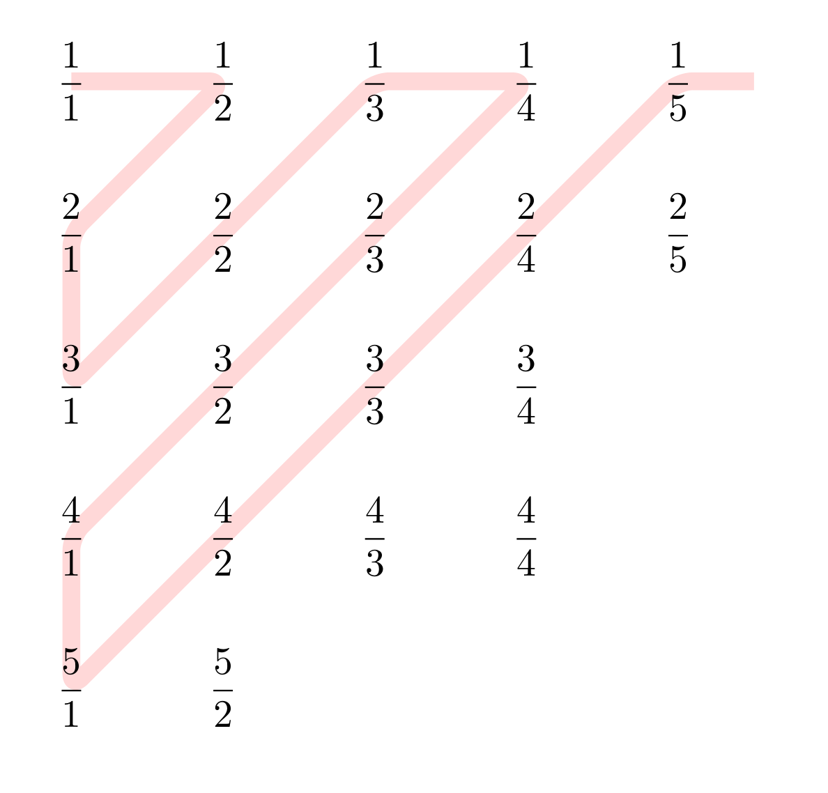
This provides an enumeration of all the positive rationals: \[ \frac{1}{1}, \frac{1}{2}, \frac{2}{1}, \frac{3}{1}, \frac{2}{2}, \frac{1}{3}, \frac{1}{4}, \frac{2}{3},\ldots \] To enumerate all rationals (positive and negative), we simply place the negative of each value immediately after it: \[ \frac{1}{1}, -\frac{1}{1}, \frac{1}{2}, -\frac{1}{2}, \frac{2}{1}, -\frac{2}{1}, \frac{3}{1}, -\frac{3}{1}, \frac{2}{2}, -\frac{2}{2}, \frac{1}{3}, -\frac{1}{3}, \frac{1}{4}, \frac{1}{4}, \frac{2}{3}, -\frac{2}{3}\ldots \] This is all standard, well-known stuff, and as far as countability goes, pretty trivial.
One might reasonably ask: is there a way of enumerating all rationals in such a way that no rational is repeated, and that every rational appears naturally in its lowest form?
Indeed there is; in fact there are several, of which one of the newest, most elegant, and simplest, is using the Calkin-Wilf tree. This is named for its discoverers (or creators, depending on which philosophy of mathematics you espouse), who described it in an article happily available on the archived web site of the second author. Herbert Wilf died in 2012, but the Mathematics Department at the University of Pennsylvania have maintained the page as he left it, as an online memorial to him.
The Calkin-Wilf tree is a binary tree with root \(a / b = 1 / 1\). From each node \(a / b\) the left child is \(a / (a+b)\) and the right child is \((a+b) / b\). From each node \(a / b\), the path back to the root contains the fractions which encode, as it were, the Euclidean algorithm for determining the greatest common divisor of \(a\) and \(b\). It is not hard to show that every fraction in the tree is in its lowest terms, and appears only once; also that every rational appears in the tree.
The enumeration of the rationals can thus be made by a breadth-first transversal of the tree; in other words listing each level of the tree one after the other:
\[ \underbrace{\frac{1}{1}}_{\text{The root}},; \underbrace{\frac{1}{2},; \frac{2}{1}}_{\text{first level}},; \underbrace{\frac{1}{3},; \frac{3}{2},; \frac{2}{3},; \frac{3}{1}}_{\text{second level}},; \underbrace{\frac{1}{4},; \frac{4}{3},; \frac{3}{5},; \frac{5}{2},; \frac{2}{5},; \frac{5}{3},; \frac{3}{4},; \frac{4}{1}}_{\text{third level}};\ldots \]
Note that the denominator of each fraction is the numerator of its successor (again, this is not hard to prove in general); thus given the sequence
\[ b_i=0,1,1,2,1,3,2,3,1,4,3,5,2,5,3,4,\ldots \]
(indexed from zero), the rationals are enumerated by \(b_i/b_{i+1}\). This sequence pre-dates Calkin and Wilf; is goes back to an older enumeration now called the Stern-Brocot tree named for the mathematician Moritz Stern and the clock-maker Achille Brocot (who was investigating gear ratios), who discovered this tree independently in the early 1860's.
The sequence \(b_i\) is called Stern's diatomic sequence and can be generated recursively:
\[ b_i=\left\{\begin{array}{ll} i,&\text{if $i\le 1$}\\\ b_{i/2},&\text{if $i$ is even}\\\ b_{(i-1)/2}+b_{(i+1)/2},&\text{if $i$ is odd} \end{array} \right. \]
Alternatively: \[ b_0=0,;b_1=1,;b_{2i}=b_i,b_{2i+1}=b_i+b_{i+1}\text{ for }i\ge 1. \] This is the form in which it appears as sequence 2487 in the OEIS.
So we can generate Stern's diatomic sequence \(b_i\), and then the successive fractions \(b_i/b_{i+1}\) will generate each rational exactly once.
If that isn't remarkable enough, sometime prior to 2003, Moshe Newman showed that the Calkin-Wilf enumeration of the rationals can in fact be done directly: \[ x_0 = 1,\quad x_{i+1}=\frac{1}{2\lfloor x_i\rfloor -x_i +1};\text{for};i\ge 1 \] will generate all the rationals. I can't find anything at all about Moshe Newman; he is always just mentioned as having "shown" this result. Never where, or to whom. There is a proof for this in an article "New Looks at Old Number Theory" by Aimeric Malter, Dierk Schleicher and Don Zagier, published in The American Mathematical Monthly , Vol. 120, No. 3 (March 2013), pp. 243-264. The part of the article relating to enumeration of rationals is based on a prize-winning mathematical essay by the first author (who at the time was a high school student in Bremen, Germany), when he was only 13. Here is the skeleton of Malter's proof:
If \(x\) is any node, then its left and right hand children are \(L = x / (x+1)\) and \(R = 1+x = 1 / (1-L)\) respectively. And clearly \(R = 1/(2\lfloor L\rfloor -L +1)\). Suppose now that \(A\) is a right child, and \(B\) is its successor rational. Then \(A\) and \(B\) will have a common ancestor \(z=p/q\), say \(k\) generations ago. To get from \(z\) to \(A\) will require one left step and \(k-1\) right steps. It is easy to show (by induction if you like), that
\[ A = k-1+\frac{p}{p+q} \] and for its successor \(B\), obtained by one right step from \(z\) and \(k-1\) left steps: \[ B = \frac{1}{\frac{q}{p+q}+k-1}. \] Since \(k-1=\lfloor A\rfloor\), and since \[ \frac{p}{p+q} = A-\lfloor A\rfloor \] it follows that \[ B=\frac{1}{1-(A-\lfloor A\rfloor))+\lfloor A\rfloor}=\frac{1}{2\lfloor A\rfloor-A+1}. \] The remaining case is moving from the end of one row to the beginning of the next, that is, from \(n\) to \(1 / (n+1)\). And this is trivial.
What's more, we can write down the isomorphisms between this sequence of positive rationals and in positive integers. Define \(N:\Bbb{Q}\to\Bbb{Z}\) as follows:
\[ N(p/q)=\left\{\begin{array}{ll} 1,&\text{if $p=q$}\\\ 2 N(p/(q-p)),&\text{if $p\lt q$}\\\ 2 N((p-q)/q)+1,&\text{if $p\gt q$} \end{array} \right. \]
Without going through a formal proof, what this does is simply count the number of steps taken to perform the Euclidean algorithm on \(p\) and \(q\). The extra factors of 2 ensure that rationals in level \(k\) have values between \(2^k\) and \(2^{k+1}\), and the final "\(+1\)" differentiates left and right children. This function assumes that \(p\) and \(q\) are relatively prime; that is, that the fraction \(p/q\) is in its lowest terms.
(The isomorphism in the other direction is given by \(k\mapsto b_k/b_{k+1}\) where \(b_k\) are the elements of Stern's diatomic sequence discussed above.)
This is just the sort of mathematics I like: simple, but surprising, and with depth. What's not to like?
Fitting the SIR model of disease to data in Julia
A few posts ago I showed how to do this in Python. Now it's Julia's turn. The data is the same: spread of influenza in a British boarding school with a population of 762. This was reported in the British Medical Journal on March 4, 1978, and you can read the original short article here.
As before we use the SIR model, with equations
\begin{align*} \frac{dS}{dt}&=-\frac{\beta IS}{N}\\\ \frac{dI}{dt}&=\frac{\beta IS}{N}-\gamma I\\\ \frac{dR}{dt}&=\gamma I \end{align*}
where \(S\), \(I\), and \(R\) are the numbers of susceptible, infected, and recovered people. This model assumes a constant population - so no births or deaths - and that once recovered, a person is immune. There are more complex models which include a changing population, as well as other disease dynamics.
The above equations can be written without the population; since it is constant, we can just write \(\beta\) instead of \(\beta/N\). The values \(\beta\) and \(\gamma\) are the parameters which affect the working of this model, their values and that of their ratio \(\beta/\gamma\) provide information of the speed of the disease spread.
As with Python, our interest will be to see if we can find values of \(\beta\) and \(\gamma\) which model the school outbreak.
We will do this in three functions. The first sets up the differential equations:
using DifferentialEquations

function SIR!(du,u,p,t)
    S,I,R = u
    β,γ = p
    du[1] = dS = -β*I*S
    du[2] = dI = β*I*S - γ*I
    du[3] = dR = γ*I
end
The next function determines the sum of squares between the data and the results of the SIR computations for given values of the parameters. Since we will put all our functions into one file, we can create the constant values outside any functions which might need them:
data = [1, 3, 6, 25, 73, 222, 294, 258, 237, 191, 125, 69, 27, 11, 4]
tspan = (0.0,14.0)
u0 = [762.0,1.0,0.0]

function ss(x)
    prob = ODEProblem(SIR!,u0,tspan,(x[1],x[2]))
    sol = solve(prob)
    sol_data = sol(0:14)[2,:]
    return(sum((sol_data - data) .^2))
end
Note that we don't have to carefully set up the problem to produce values at
each of the data points, which in our case are the integers from 0 to 14. Julia
will use a standard numerical technique with a dynamic step size, and values
corresponding to the data points can then be found by interpolation. All of
this functionality is provided by the DifferentialEquations package. For
example, R[10] will return the 10th value of the list of computed R values,
but R(10) will produce the interpolated value of R at \(t=10\).
Finally we use the Optim package to minimize the sum of squares, and the
Plots package to plot the result:
using Optim
using Plots

function run_optim()
    opt = optimize(ss,[0.001,0.01],NelderMead())
    beta,gamma = opt.minimizer
    prob = ODEProblem(SIR!,u0,tspan,(beta,gamma))
    sol = solve(prob)
    plot(sol,
	    linewidth=2,
	    xaxis="Time in days",
	    label=["Susceptible" "Infected" "Recovered"])
    plot!([0:14],data,linestyle=:dash,marker=:circle,markersize=4,label="Data")
end
Running the last function will produce values
\begin{align*} \beta&=0.0021806887934782853\\\ \gamma&=0.4452595474326912 \end{align*}
and the final plot looks like this:
This was at least as easy as in Python, and with a few extra bells and whistles, such as interpolation of data points. Nice!
The Butera-Pernici algorithm (2)
The purpose of this post will be to see if we can implement the algorithm in Julia, and thus leverage Julia's very fast execution time.
We are working with polynomials defined on nilpotent variables, which means that
the degree of any generator in a polynomial term will be 0 or 1. Assume that
our generators are indexed from zero: \(x_0,x_1,\ldots,x_{n-1}\), then any term in a
polynomial will have the form
\[
cx_{i_1}x_{i_2}\cdots x_{i_k}
\]
where \(\{x_{i_1}, x_{i_2},\ldots, x_{i_k}\}\subseteq\{0,1,2,\ldots,n-1\}\). We can
then express this term as an element of a dictionary {k => v} where
\[
k = 2^{i_1}+2^{i_2}+\cdots+2^{i_k}.
\]
So, for example, the polynomial term \(7x_2x_3x_5\) would correspond to the dictionary term
44 => 7
since \(44 = 2^2+2^3+2^5\). Two polynomial terms {k1 => v1} and {k2 => v2}
with no variables in common can then be multiplied simply by adding the k terms,
and multiplying the v values, to obtain {k1+k2 => v1*v2} . And we can check if
k1 and k2 have a common variable easily by evaluating k1 & k2; a non-zero
value indicates a common variable. This leads to the following Julia function
for multiplying two such dictionaries:
function poly_dict_mul(p1, p2)
  p3 = Dict{BigInt,BigInt}()
  for (k1, v1) in p1
    for (k2, v2) in p2
	  if k1 & k2 > 0
	    continue
	  else
	    if k1 + k2 in keys(p3)
		  p3[k1+k2] += v1 * v2
	    else
		  p3[k1+k2] = v1 * v2
	    end
	  end
    end
    end
  return (p3)
end
As you see, this is a simple double loop over the terms in each polynomial
dictionary. If two terms have a non-zero conjunction, we simply move on. If
two terms when added already exist in the new dictionary, we add to that term.
If the sum of terms is new, we create a new dictionary element. The use of
BigInt is to ensure that no matter how big the terms and coefficients become,
we don't suffer from arithmetic overflow.
For example, suppose we consider the product \[ (x_0+x_1+x_2)(x_1+x_2+x_3). \] A straightforward expansion produces \[ x_0x_3 + x_1x_3 + x_1^2 + x_0x_1 + x_0x_2 + 2x_1x_2 + x_2^2 + x_2x_3. \] which by nilpotency becomes \[ x_0x_3 + x_1x_3 + x_0x_1 + x_0x_2 + 2x_1x_2 + x_2x_3. \] The dictionaries corresponding to the two polynomials are
{1 => 1, 2 => 1, 4 => 1}
and
{2 => 1, 4 => 1, 8 => 1}
Then:
julia> poly_dict_mul(Dict(1=>1,2=>1,4=>1),Dict(2=>1,4=>1,8=>1))
Dict{BigInt,BigInt} with 6 entries:
  9  => 1
  10 => 1
  3  => 1
  5  => 1
  6  => 2
  12 => 1
If we were to rewrite the keys as binary numbers, we would have
{1001 => 1, 1010 => 1, 11 => 1, 101 => 1, 110 => 2, 1100 => 1}
in which you can see that each term corresponds with the term of the product above.
Having conquered multiplication, finding the permanent should then require two steps:
- Turning each row of the matrix into a polynomial dictionary.
- Starting with \(p=1\), multiply all rows together, one at a time.
For step 1, suppose we have a row \(i\) of a matrix \(M=m_{ij}\). Then starting
with an empty dictionary p, we move along the row, and for each non-zero element
\(m_{ij}\) we add the term p[BigInt(1)<<j] = M[i,j]. For speed we use bit
operations instead of arithmetic operations. This means we can create a list of
all polynomial dictionaries:
function mat_polys(M)
  (n,ncols) = size(M)
  ps = []
  for i in 1:n
    p = Dict{BigInt,BigInt}()
    for j in 1:n
      if M[i,j] == 0
	    continue
      else
	    p[BigInt(1)<<(j-1)] = M[i,j]
      end
    end
    push!(ps,p)
  end
  return(ps)
end
Step 2 is a simple loop; the permanent will be given as the value in the final step:
function poly_perm(M)
  (n,ncols) = size(M)
  mp = mat_polys(M)
  p = Dict{BigInt,BigInt}(0=>1)
  for i in 1:n
    p = poly_dict_mul(p,mp[i])
  end
  return(collect(values(p))[1])
end
We don't in fact need two separate functions here; since the polynomial dictionary for each row is only used once, we could simply create each one as we needed. However, given that none of our matrices will be too large, the saving of time and space would be minimal.
Now for a few tests:
julia> n = 10; M = [BigInt(1)*mod(j-i,n) in [1,2,3] for i = 1:n, j = 1:n);
julia> poly_perm(M)
125

julia> n = 20; M = [BigInt(1)*mod(j-i,n) in [1,2,3] for i = 1:n, j = 1:n);
julia> @time poly_perm(M)
  0.003214 seconds (30.65 k allocations: 690.875 KiB)
15129

julia> n = 40; M = [BigInt(1)*mod(j-i,n) in [1,2,3] for i = 1:n, j = 1:n);
julia> @time poly_perm(M)
  0.014794 seconds (234.01 k allocations: 5.046 MiB)
228826129

julia> n = 100; M = [BigInt(1)*mod(j-i,n) in [1,2,3] for i = 1:n, j = 1:n);
julia> @time poly_perm(M)
  0.454841 seconds (3.84 M allocations: 83.730 MiB, 27.98% gc time)
792070839848372253129

julia> lucasnum(n)+2
792070839848372253129
This is extraordinarily fast, especially compared with our previous attempts: naive attempts using all permutations, and using Ryser's algorithm.
- A few comparisons
Over the previous blog posts, we have explored various different methods of
computing the permanent:

-   `permanent`, which is the most naive method, using the formal definition, and
    summing over all the permutations \\(S\_n\\).

-   `perm1`, Ryser's algorithm, using the Combinatorics package and iterating over
    all non-empty subsets of \\(\\{1,2,\ldots,n\\}\\).

-   `perm2`, Same as `perm1` but instead of using subsets, we use all non-zero
    binary vectors of length n.

-   `perm3`, Ryser's algorithm using Gray codes to speed the transition between
    subsets, and using a lookup table.

All these are completely general, and aside from the first function, which is
the most inefficient, can be used for any matrix up to size about \\(25\times 25\\).

So consider the \\(n\times n\\) circulant matrix with three ones in each row, whose
permanent is \\(L(n)+2\\).  The following table shows times in seconds (except where
minutes is used) for each calculation:

<style>.table-nocaption table { width: 75%;  text-align: left;  }</style>

<div class="ox-hugo-table table-nocaption">
<div></div>

|             | 10     | 12    | 15    | 20    | 30    | 40   | 60   | 100  |
|-------------|--------|-------|-------|-------|-------|------|------|------|
| `permanent` | 9.3    | -     | -     | -     | -     | -    | -    | -    |
| `perm1`     | 0.014  | 0.18  | 0.72  | 47    | -     | -    | -    | -    |
| `perm2`     | 0.03   | 0.105 | 2.63  | 166   | -     | -    | -    | -    |
| `perm3`     | 0.004  | 0.016 | 0.15  | 12.4  | -     | -    | -    | -    |
| `poly_perm` | 0.0008 | 0.004 | 0.001 | 0.009 | 0.008 | 0.02 | 0.05 | 0.18 |

</div>

Assuming that the time taken for `permanent` is roughly proportional to \\(n!n\\),
then we would expect that the time for matrices of sizes 23 and 24 would be
about \\(1.5\times 10^{17}\\) and \\(3.8\times 10^{18}\\) seconds respectively.  Note
that the age of the universe is approximately \\(4.32\times 10^{17}\\) seconds, so
my laptop would need to run for about the third of the universe's age to compute
the permanent of a \\(23\times 23\\) matrix.  That's about the time since the solar
system and the Earth were formed.

Note also that `poly_perm` will slow down if the number of non-zero values in
each row increases.  For example, with four consecutive ones in each row, it
takes over 10 seconds for a \\(100\times 100\\) matrix.  With five ones in each row,
it takes about 2.7 and 21.6 seconds respectively for matrices of size 40 and 60.
Extrapolating indicates that it would take about 250 seconds for the \\(100\times
100\\) matrix.  In general, an \\(n\times n\\) matrix with \\(k\\) non-zero elements in
each row will have a time complexity approximately of order \\(n^k\\).  However,
including the extra optimization (which we haven't done) that allows for
elements to be set to one before the multiplication, produces an algorithm whose
complexity is \\(O(2^{\text{min}(2w,n)}(w+1)n^2)\\) where \\(n\\) is the size of the
matrix, and \\(w\\) its band-width.  See the [original
paper](<https://arxiv.org/abs/1406.5337>) for details.
The Butera-Pernici algorithm (1)
Introduction
We know that there is no general sub-exponential algorithm for computing the permanent of a square matrix. But we may very reasonably ask -- might there be a faster, possibly even polynomial-time algorithm, for some specific classes of matrices? For example, a sparse matrix will have most terms of the permanent zero -- can this be somehow leveraged for a better algorithm?
The answer seems to be a qualified "yes". In particular, if a matrix is banded, so that most diagonals are zero, then a very fast algorithm can be applied. This algorithm is described in an online article by Paolo Butera and Mario Pernici called Sums of permanental minors using Grassmann algebra. Accompanying software (Python programs) is available at github. This software has been rewritten for the SageMath system, and you can read about it in the documentation. The algorithm as described by Butera and Pernici, and as implemented in Sage, actually produces a generating function.
Our intention here is to investigate a simpler version, which computes the permanent only.
Basic outline
Let \(M\) be an \(n\times n\) square matrix, and consider the polynomial ring on \(n\) variables \(x_1,x_2,\ldots,x_n\). Each row of the matrix will correspond to an element of this ring; in particular row \(i\) will correspond to
\[ \sum_{j=1}^nm_{ij}a_j=m_{i1}a_1+m_{i2}a_2+\cdots+m_{in}a_n. \]
Suppose further that all the generating elements \(x_i\) are nilpotent of order two, so that \(x_i^2=0\).
Now if we take all the row polynomials and multiply them, each term of the product will have order \(n\). But by nilpotency, all terms which contain a repeated element will vanish. The result will be only those terms which contain each generator exactly once, of which there will be \(n!\). To obtain the permanent all that is required is to set \(x_i=1\) for each generator.
Here's an example in Sage.
sage: R.<a,b,c,d,e,f,g,h,i,x1,x2,x3> = PolynomialRing(QQbar)
sage: M = matrix([[a,b,c],[d,e,f],[g,h,i]])
sage: X = matrix([[x1],[x2],[x3]])
sage: MX = M*X

[a*x1 + b*x2 + c*x3]
[d*x1 + e*x2 + f*x3]
[g*x1 + h*x2 + i*x3]
To implement nilpotency, it's easiest to reduce modulo the ideal defined by \(x_i^2=0\) for all \(i\). So we take the product of those row elements, and reduce:
sage: I = R.ideal([x1^2, x2^2, x3^2])
sage: pr = MX[0,0]*MX[1,0]*MX[2,0]
sage: pr.reduce(I)

c*e*g*x1*x2*x3 + b*f*g*x1*x2*x3 + c*d*h*x1*x2*x3 + a*f*h*x1*x2*x3 + b*d*i*x1*x2*x3 + a*e*i*x1*x2*x3
Finally, set each generator equal to 1:
sage: pr.reduce(I).subs({x1:1, x2:1, x3:1})

c*e*g + b*f*g + c*d*h + a*f*h + b*d*i + a*e*i
and this is indeed the permanent for a general \(3\times 3\) matrix.
Some experiments
Let's experiment now with the matrices we've seen in a previous post, which contain three consecutive super-diagonals of ones, and the rest zero.
Such a matrix is easy to set up in Sage:
sage: n = 10
sage: v = n*[0]; v[1:4] = [1,1,1]
sage: M = matrix.circulant(v)
sage: M

[0 1 1 1 0 0 0 0 0 0]
[0 0 1 1 1 0 0 0 0 0]
[0 0 0 1 1 1 0 0 0 0]
[0 0 0 0 1 1 1 0 0 0]
[0 0 0 0 0 1 1 1 0 0]
[0 0 0 0 0 0 1 1 1 0]
[0 0 0 0 0 0 0 1 1 1]
[1 0 0 0 0 0 0 0 1 1]
[1 1 0 0 0 0 0 0 0 1]
[1 1 1 0 0 0 0 0 0 0]
Similarly we can define the polynomial ring:
sage: R = PolynomialRing(QQbar,x,n)
sage: R.inject_variables()

Defining x0, x1, x2, x3, x4, x5, x6, x7, x8, x9
And now the polynomials corresponding to the rows:
sage: MX = M*matrix(R.gens()).transpose()
sage: MX

[x1 + x2 + x3]
[x2 + x3 + x4]
[x3 + x4 + x5]
[x4 + x5 + x6]
[x5 + x6 + x7]
[x6 + x7 + x8]
[x7 + x8 + x9]
[x0 + x8 + x9]
[x0 + x1 + x9]
[x0 + x1 + x2]
If we multiply them, we will end up with a huge expression, far too long to display:
sage: pr = prod(MX[i,0] for i in range(n))
sage: len(pr.monomials)

14103
We could reduce this by the ideal, but that would be slow. Far better to reduce after each separate multiplication:
sage: I = R.ideal([v^2 for v in R.gens()])
sage: p = R.one()
sage: for i in range(n):
	      p = p*MX[i,0]
	      p = p.reduce(I)

sage: p.subs({v:1 for v in R.gens())
125
The answer is almost instantaneous. We can repeat the above list of commands
starting with different values of n; for example with n=20 the result is 15129,
as we expect.
This is not yet optimal; for n=20 on my machine the final loop takes about 7.8 seconds. Butera and Pernici show that the multiplication and setting the variables to one can sometimes be done in the opposite order; that is, some variables can be identified to be set to one before the multiplication. This can speed the entire loop dramatically, and this optimization has been included in the Sage implementation. For details, see their paper.
The size of the universe
As a first blog post for 2020, I'm dusting off one from my previous blog, which I've edited only slightly.
I've been looking up at the sky at night recently, and thinking about the sizes of things. Now it's all very well to say something is for example a million kilometres away; that's just a number, and as far as the real numbers go, a pretty small one (all finite numbers are "small"). The difficulty comes in trying to marry very large distances and times with our own human scale. I suppose if you're a cosmologist or astrophysicist this is trivial, but for the rest of us it's pretty daunting.
It's all a problem of scale. You can say the sun has an average distance of 149.6 million kilometres from earth (roughly 93 million miles), but how big, really, is that? I don't have any sense of how big such a distance is: my own sense of scale goes down to about 1mm in one direction, and up to about 1000km in the other. This is hopelessly inadequate for cosmological measurements.
So let's start with some numbers:
-
Diameter of Earth: 12,742 km
-
Diameter of the moon: 3,475km
-
Diameter of Sun: 1,391,684 km
-
Diameter of Jupiter: 139,822 km
-
Average distance of Earth to the sun: 149,597,870km
-
Average distance of Jupiter to the sun: 778.5 million km
-
Average distance of Earth to the moon: 384,400 km
Of course since all orbits are elliptical, distances will both exceed and be less than the average at different times. However, for our purposes of scale, an average is quite sufficient.
By doing a bit of division, we find that the moon is about 0.27 the width of the earth, Jupiter is about 11 times bigger (in linear measurements) and the Sun about 109.2 times bigger than the Earth.
Now for some scaling. We will scale the earth down to the size of a mustard seed, which is about 1mm in diameter. On this scale, the Sun is about the size of a large grapefruit (which happily is large, round, and yellow), and the moon is about the size of a dust mite:
On this new scale, with 12742 km equals 1 millimetre, the above distances become:
-
Diameter of Earth: 1mm
-
Diameter of the moon: 0.27mm
-
Diameter of Sun: 109.2m
-
Diameter of Jupiter: 10.97mm
-
Average distance of Earth to the sun: 11740mm = 11.74m
-
Average distance of Jupiter to the sun: 61097.2mm = 61.1m
-
Average distance of Earth to the moon: 30.2mm = 3cm
So how long is the distance from the sun to the Earth? Well, a cricket pitch is 22 yards long, so 11 yards from centre to end, which is about 10.1 metres. So imagine our grapefruit placed at the centre of a cricket pitch. Go to an end of the pitch, and about 1.5 metres (about 5 feet) beyond. Place the mustard seed there. What you now have is a scale model of the sun and earth.
Here's a cricket pitch to give you an idea of its size:
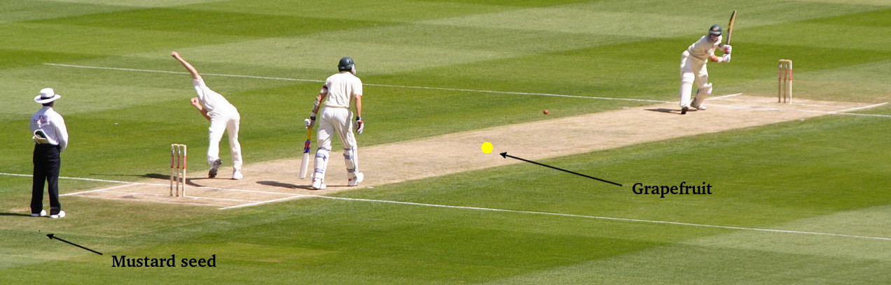
Note that in this picture, the yellow circle is not drawn to size. If you look just left of centre, you'll see the cricket ball, which has a diameter of about 73mm. Our "Sun" grapefruit should be about half again as wide as that.
If you don't have a sense of a cricket pitch (even with this picture), consider instead a tennis court: the distance from the net to the baseline is 39 feet, or 11.9m. At our scale, this is nearly exact:
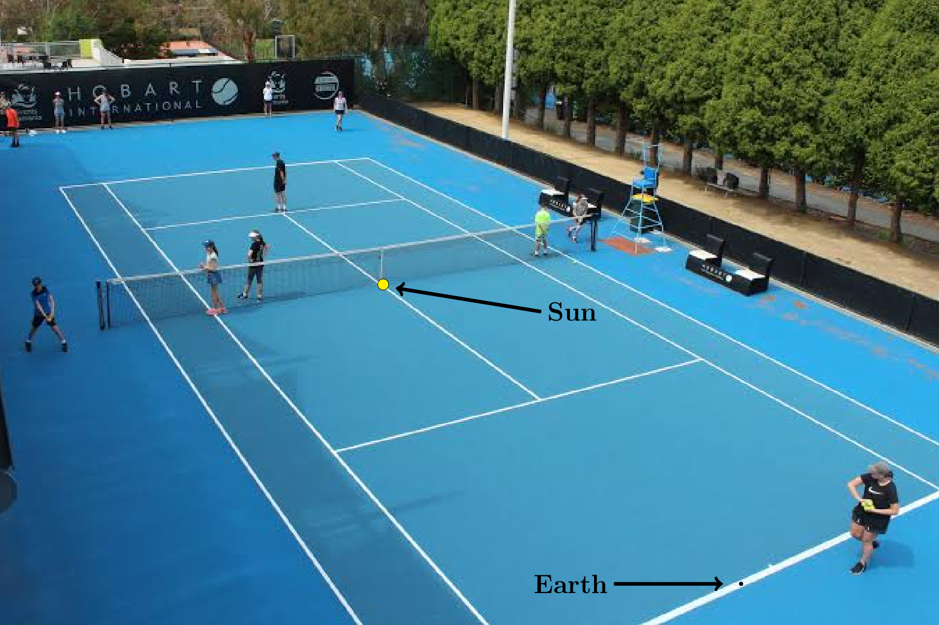
(Note that on this scale the sun is somewhat bigger than a tennis ball, and the Earth would in fact be too small to see on this picture.)
So we now have a scale model of the Sun and Earth. If we wanted to include the Moon, start with its average distance from Earth (384,400 km), then we'd have a dust mite circling our mustard seed at a distance of 3cm.
How about Jupiter? Well, we noted before that it is about 61m away. Continuing with our cricket pitch analogy, imagine three pitches laid end to end, which is 66 yards, or 60.35 metres. Not too far off, really! So place the grapefruit at the end of the first pitch, the mustard seed a little away from centre, and at the end of the third pitch place an 11mm ball for Jupiter: a glass marble will do nicely for this.
And the size of the solar system? Assuming the edge is given by the heliopause (where the Sun's solar wind is slowed down by interstellar particles); this is at a distance of about 18,100,000,000 km from the Sun, which in our scale is about 1.42 km, or a bit less than a mile (0.88 miles). Get that? With Earth the size of a mustard seed, the edge of the solar system is nearly a mile away!
Onwards and outwards
So with this scaling we have got the solar system down to a reasonably manageable size. If 149,600,000 km seems too vast a distance to make much sense of, scaling it down to 11.7 metres is a lot easier. But let's get cosmological here, and start with a light year, which is 9,460,730,472,580,800 m, or more simply (and inexactly) 9.46× 10¹⁵m. In our scale, that becomes 742,483,948.562 mm, or about 742 km, which is about 461 miles. That's about the distance from New York city to Greensboro, NC, or from Melbourne to Sydney. The nearest star is Proxima Centauri, which is 4.3 light years away: at our Earth=mustard seed scale, that's about 3192.6 km, or 1983.8 miles. This is the flight distance from Los Angeles to Detroit. Look at that distance on an atlas, imagine our planet home mustard seed at one place and consider getting to the other.
The furthest any human has been from the mustard seed Earth is to the dust-mite Moon: 3cm, or 1.2 inches away. To get to the nearest star is, well, a lot further!
The nearest galaxy to the Milky Way is about 0.025 mly away. ("mly" = "millions of light years"). Now we're getting into the big stuff. At our scale, this distance will be 18,500,000 kilometres, which means that at our mustard seed scale, the nearest galaxy is about 18.5 million kilometres away. And there are lots of other galaxies, and much further away than this. For example, the Andromeda Galaxy is 2,538,000 light years away, which at our scale is 1,884,465,000 km -- nearly two billion kilometres!
What's remarkable is that even scaling the Earth down to a tiny mustard seed speck, we are still up against distances too vast for human scale. We could try scaling the Earth down to a ball whose diameter is the thickness of the finest human hair -- about 0.01 mm -- which is the smallest distance within reach of our own scale. But even at this scale distances are only reduced by a factor of 100, so the nearest galaxy is still 18,844,650 km away.
One last try: suppose we scale the entire Solar System, out to the heliopause, down to a mustard seed. This means that the diameter of the heliopause: 36,200,000,000 km, is scaled down to 1mm. Note that the heliopause is about three times further away from the sun than the mean distance of Pluto. At this scale, one light year is a happily manageable 261mm, or about ten and a quarter inches. So the nearest star is 1.12m away, or about 44 inches. And the nearest galaxy? Well, it's 25000 light years away, which puts it at about 6.5 km. The Andromeda Galaxy is somewhat over 663 km away. The furthest galaxy, with the enticing name of GN-z11 is said to be about 34 billion light years away. On our heliopause=mustard seed scale, that's about 9.1 million kilometres.
There's no escaping it, the Universe is big, and the scales need to describe it, no matter how you approach them, quickly leap out of of our own human scale.
Permanents and Ryser's algorithm
As I discussed in my last blog post, the permanent of an \(n\times n\) matrix \(M=m_{ij}\) is defined as \[ \text{per}(M)=\sum_{\sigma\in S_n}\prod_{i=1}^nm_{i,\sigma(i)} \] where the sum is taken over all permutations of the \(n\) numbers \(1,2,\ldots,n\). It differs from the better known determinant in having no sign changes. For example: \[ \text{per} \begin{bmatrix}a&b&c\\d&e&f\\g&h&i\end{bmatrix} =aei+afh+bfg+bdi+cdi+ceg. \] By comparison, here is the determinant: \[ \text{det} \begin{bmatrix}a&b&c\\d&e&f\\g&h&i\end{bmatrix} =aei - afh + bfg - bdi + cdi - ceg. \] The apparent simplicity of the permanent definition hides the fact that there is no known sub-exponential algorithm to compute it, nor does it satisfy most of the nice properties of determinants. For example, we have
\[ \text{det}(AB)=\text{det}(A)\text{det}(B) \]
but in general \(\text{per}(AB)\ne\text{per}(A)\text{per}(B)\). Nor is the permanent zero if two rows are equal, or if any subset of rows is linearly dependent.
Applying the definition and summing over all the permutations is prohibitively slow; of \(O(n!n)\) complexity, and unusable except for very small matrices.
In the small but excellent textbook "Combinatorial Mathematics" by Herbert J. Ryser and published in 1963, one chapter is devoted to the inclusion-exclusion principle, of which the computation of permanents is given as an example. The permanent may be considered as a sum of products, where in each product we choose one value from each row and one value from each column.
Suppose we start by adding the rows together and multiplying them: \[ P = (a+d+g)(b+e+h)(c+f+i). \] This will certainly contain all elements of the permanent, but it also includes products we don't want, such as for example \(aef\) where the elements are chosen from only two rows, and \(ghi\) where the elements are all in one row.
To eliminate all possible products from only two rows we subtract them:
\begin{align*} P & -(a+d)(b+e)(c+f)\text{ rows $1$ and $2$}\\\ & - (a+g)(b+h)(c+i)\text{ rows $1$ and $3$}\\\ & - (d+g)(e+h)(f+i)\text{ rows $2$ and $3$} \end{align*}
The trouble with that subtraction is that we are subtracting products of each individual row twice; for example \(abc\) is in the first and second products. But we only want to subtract those products once from \(P\). So we have to add them again:
\begin{align*} P & -(a+d)(b+e)(c+f)\qquad\text{ rows $1$ and $2$}\\\ & - (a+g)(b+h)(c+i)\qquad\text{ rows $1$ and $3$}\\\ & - (d+g)(e+h)(f+i)\qquad\text{ rows $2$ and $3$}\\\ & + abc\\\ & + def\\\ & + ghi. \end{align*}
Computing the permanent of a \(4\times 4\) matrix would start by adding all the rows and multiplying the sums. Then we would subtract all products of rows taken three at a time. But this would subtract all products of rows taken two at a time twice for each pair, so we add those products back in again. Finally we find that the number of times we've subtracted products of a single row have cancelled out, so we need to subtract them again:
\begin{array}{ccccc} &1&2&3&4\\\ -&1&2&3&\\\ -&1&2&&4\\\ -&1&&3&4\\\ -&&2&3&4\\\ +&1&2&&\\\ +&1&&3&\\\ +&1&&&4\\\ +&&2&3&\\\ +&&2&3&\\\ +&&&3&4\\\ -&1\\\ -&&2\\\ -&&&3\\\ -&&&&4 \end{array}
After all of this we are left with only those products which include all fours rows and columns. And as you see, this is a standard inclusion-exclusion approach.
For an \(n\times n\) matrix, let \(S=\{1,2,\ldots,n\}\), and let \(X\subseteq S\). Then define \(R(X)\) to be the product of the sums of elements of rows indexed by \(X\). For example, with \(S=\{1,2,3\}\) and \(X=\{1,3\}\), then
\[ R(X)=(a+g)(b+h)(c+i). \] We can thus write the above method for obtaining the permanent as:
\begin{align*} \text{per}(M)&=\sum_{\emptyset\ne X\subseteq S}(-1)^{n-|X|}R(X)\\\ &= (-1)^n\sum_{\emptyset\ne X\subseteq S}(-1)^{|X|}R(X) \end{align*}
This is Ryser's algorithm.
Naive Implementation
A naive implementation would be to simply iterate through all the non-empty subsets \(X\) of \(S=\{1,2,\ldots,n\}\), and for each subset add those rows, and multiply the resulting sums.
Here's one such Julia function:
using Combinatorics

function perm1(M)
    n, nc = size(M)
    S = 1:n
    P = 0
    for X in setdiff(powerset(S),powerset([]))
	    P += (-1)^length(X)*prod(sum(M[i,:] for i in X))
    end
    return((-1)^n * P)
end
Alternatively, we can manage without any extra packages, and use the fact that the subsets of \(S\) correspond to the binary digits of integers between 1 and \(2^n-1\):
function perm2(M)
    n,nc = size(m)
    P = 0
    for i in (1:2^n-1)
	    indx = digits(i,base=2,pad=n)
	    P += (-1)^sum(indx)*prod(sum(M .* indx,dims=1))
    end
    return((-1)^n * P)
end
Now for some tests. There are very few matrices for which the permanent has a known value; however there are some circulant matrices of zeros and ones whose permanent is known. One such is the \(n\times n\) matrix \(M=m_{ij}\) whose first, second, and third circulant superdiagonals are ones; that is, for which
\[ m_{ij}=1 \Leftrightarrow\bmod(j-1,n)\in\{1,2,3\}. \]
(Note that since the permanent is trivially unchanged by any permutation of the rows, \(M\) can be also defined as being a circulant matrix each row of which has three consecutive ones.)
Then
\[ \text{per}(M)=F_{n-1}+F_{n+1}+2 \]
where \(F_k\) is the \(k\) -th Fibonacci number indexed from 1, so that \(F_1=F_2=1\). Note that the sums of Fibonacci numbers whose indices differ by two form the Lucas numbers \(L_n\).
Alternatively,
\[ \text{per}(M)=\text{trace}(C_2^n)+2 \]
where
\[ C_2=\begin{bmatrix}0&1\\1&1\end{bmatrix} \]
This result, and some others, can be found in the article "Permanents" by Marvin Marcus and Henryk Minc, in The American Mathematical Monthly, Vol. 72, No. 6 (Jun. - Jul., 1965), pp. 577-591.
julia> n = 10;

julia> M = [1*(mod(j-i,n) in [1,2,3]) for i=1:n, j=1:n]
10×10 Array{Int64,2}:
 0  1  1  1  0  0  0  0  0  0
 0  0  1  1  1  0  0  0  0  0
 0  0  0  1  1  1  0  0  0  0
 0  0  0  0  1  1  1  0  0  0
 0  0  0  0  0  1  1  1  0  0
 0  0  0  0  0  0  1  1  1  0
 0  0  0  0  0  0  0  1  1  1
 1  0  0  0  0  0  0  0  1  1
 1  1  0  0  0  0  0  0  0  1
 1  1  1  0  0  0  0  0  0  0

julia> perm1(M)
125

julia> perm2(M)
125

julia> fibonaccinum(n-1)+fibonaccinum(n+1)+2
125

julia> lucasnum(n)+2
125

julia> C2=[0 1; 1 1];

julia> tr(C2^n)+2
125
However, it seems that using the machinery of subsets adds to the time, which becomes noticeable if \(n\) is large:
julia> using Benchmarktools

julia> n = 20; M = [1*(mod(j-i,n) in [1,2,3]) for i=1:n, j=1:n];

julia> @time perm1(M)
  6.703187 seconds (31.46 M allocations: 5.097 GiB, 17.93% gc time)
15129

julia> @time perm2(M)
  1.677242 seconds (3.21 M allocations: 3.721 GiB, 8.69% gc time)
15129
That is, the perm2 implementation is about four times faster than perm1.
Implementation with Gray codes
Here is where we can show some cleverness. Recall that a Gray code is a listing of all numbers 0 through \(2^n-1\) whose binary expansion changes in only one bit between consecutive values. It is also known that for \(1\le k\le 2^n-1\) then the Gray code corresponding to \(k\) is given by \(k\oplus (k\gg 1)\). For example, for \(n=4\):
julia> for i in 1:15
       j = xor(i,i>>1)
       println(lpad(i,2),":\t\b\b\b",bin(i,4),'\t',lpad(j,2),":\t\b\b\b",bin(j,4))
       end
 1:  [1, 0, 0, 0]        1:  [1, 0, 0, 0]
 2:  [0, 1, 0, 0]        3:  [1, 1, 0, 0]
 3:  [1, 1, 0, 0]        2:  [0, 1, 0, 0]
 4:  [0, 0, 1, 0]        6:  [0, 1, 1, 0]
 5:  [1, 0, 1, 0]        7:  [1, 1, 1, 0]
 6:  [0, 1, 1, 0]        5:  [1, 0, 1, 0]
 7:  [1, 1, 1, 0]        4:  [0, 0, 1, 0]
 8:  [0, 0, 0, 1]       12:  [0, 0, 1, 1]
 9:  [1, 0, 0, 1]       13:  [1, 0, 1, 1]
10:  [0, 1, 0, 1]       15:  [1, 1, 1, 1]
11:  [1, 1, 0, 1]       14:  [0, 1, 1, 1]
12:  [0, 0, 1, 1]       10:  [0, 1, 0, 1]
13:  [1, 0, 1, 1]       11:  [1, 1, 0, 1]
14:  [0, 1, 1, 1]        9:  [1, 0, 0, 1]
15:  [1, 1, 1, 1]        8:  [0, 0, 0, 1]
Note that in the rightmost column of binary expansions, there is only one bit shift between consecutive values: either a single 1 is added, or removed.
For Ryser's algorithm, we can consider this in terms of our sum of rows: if the subsets are given in Gray code order, then moving from one subset to the next is a matter of just adding or subtracting one row from the current sum.
We are not so much interested in the codes themselves, as in their successive differences. For example here are the differences for \(n=4\):
julia> [xor(k,k>>1)-xor(k-1,(k-1)>>1) for k in 1:15]'
1×14 Adjoint{Int64,Array{Int64,1}}:
 1  2  -1  4  1  -2  -1  8  1  2  -1  -4  1  -2  -1
This sequence is A055975 in the Online Encyclopaedia of Integer Sequences, and can be computed as
\[ a[n] = \begin{cases} n,&\text{if $n\le 2$}\\\ 2a[n/2],&\text{if $n$ is even}\\\ (-1)^{(n-1)/2},&\text{if $n$ is odd} \end{cases} \]
We can interpret each term in this sequence as the row that should be added or subtracted from the current sum. A value of \(2^m\) means adding row \(m+1\); a value of \(-2^m\) means subtracting row \(m+1\). From any difference, we can obtain the bit position by taking the logarithm to base 2, and whether to add or subtract by its sign. But in fact the number of differences is very small: only \(2n\), so it will be much easier to create a lookup table, using a dictionary:
v = vcat([(2^i,i+1,1) for i in 0:n-1],[(-2^i,i+1,-1) for i in 0:n-1])
lut = Dict(x[1] => (x[2],x[3]) for x in v)
For example, for \(n=3\) the lookup dictionary is
4  => (3, 1)
-4 => (3, -1)
2  => (2, 1)
-2 => (2, -1)
-1 => (1, -1)
1  => (1, 1)
Now we can implement the algorithm by first pre-computing the sequences of differences, and for each element of the sequence, use the lookup dictionary to determine what row is to be added or subtracted. We start with the first row.
Putting all this together gives another implementation of the permanent:
function perm3(M) # Gray code version with lookup tables
    n,nc = size(M)
    if n != nc
	    error("Matrix must be square")
    end
    gd = zeros(Int64,1,2^n-1)
    gd[1] = 1

    v = vcat([(2^i,i+1,1) for i in 0:n-1],[(-2^i,i+1,-1) for i in 0:n-1])
    lut = Dict(x[1] => (x[2],x[3]) for x in v)

    r = M[1,:] # r will contain the sum of rows
    s = -1
    pm = s*prod(r)
    for i in (2:2^n-1)
	    if iseven(i)
		    gd[i] = 2*gd[div(i,2)]
	    else
		    gd[i] = (-1)^((i-1)/2)
	    end
	    r += M[lut[gd[i]][1],:]*lut[gd[i]][2]
	    s *= -1
	    pm += s*prod(r)
    end
    return(pm * (-1)^n)
end
This can be timed as before:
julia> @time perm3(M)
  0.943328 seconds (3.15 M allocations: 728.004 MiB, 15.91% gc time)
15129
This is our best time yet.
Speeds of Julia and Python
Introduction
Python is of course one of the world's currently most popular languages, and there are plenty of statistics to show it. Of all languages in current use, Python is one of the oldest (in the very quick time-scale of programming languages) dating from 1990 - only C and its variants are older. However, it seems to keep its eternal youth by being re-invented, and by its constantly increasing libraries. Indeed, one of Python's greatest strength is its libraries, and pretty much every Python user will have worked with numpy, scipy, matplotlib, pandas, to name but four. In fact, aside from some specialized applications (mainly involving security, speed, or memory) Python can be happily used for almost everything.
Julia on the other hand is newer, dating from 2012. (Only Swift is newer.) It was designed to have the speed of C, the power of Matlab, and the ease of use of Python. Note the comparison with Matlab - Julia was designed as a language for technical computing, although it is very much a general purpose language. It can even be used for low-level systems programming.
Like Python, Julia can be extended through packages, of which there are many: according to Julia's package repository there are 2554 at the time of writing. Some of the packages are big, mature, and robust, others are smaller or represent a niche interest. You can go to Julia Observer to get a sense of which packages are the most popular, largest, have the most commits on github, and so on. Because Julia is still relatively new, packages are still being actively developed. However, some such as Plots, JuMP for optimization, Differential Equations, to name but three, are very much ready for the Big Time.
The purpose of this post is to do a single comparison of Julia and Python for speed.
Matrix permanents
Given a square matrix, its determinant is a well-known and useful construct (in spite of Sheldon Axler).
The determinant of an \(n\times n\) matrix \(M=m_{ij}\) can be formally defined as
\[ \det(M)=\sum_{\sigma\in S_n}\left(\text{sgn}(\sigma)\prod_{i=1}^nm_{i,\sigma(i)}\right) \]
where the sum is taken over all permutations \(\sigma\) of \(1,2,\ldots,n\), and where \(\text{sgn}(\sigma)\) is the sign of the permutation; which is defined in terms of the number of digit swaps to get to it: an even number of swaps has a sign of 1, and an odd number a sign of \(-1\). The determinant can be effectively computed by Gaussian elimination of a matrix into triangular form, which takes in the order of \(n^3\) operations; the determinant is then the product of the diagonal elements.
The permanent is defined similarly, except for the sign:
\[ \text{per}(M)=\sum_{\sigma\in S_n}\prod_{i=1}^nm_{i,\sigma(i)}. \]
Remarkably enough, this simple change renders the permanent impossible to be computed effectively; all known algorithms have exponential orders. Computing by expanding each permutation takes \(O(n!n)\) operations, some better algorithms (such as Ryser's algorithm) have order \(O(2^{n-1}n)\).
The permanent has some applications, although not as many as the determinant. An easy and immediate result is that if \(M\) is a matrix consisting entirely of ones, except for the main diagonal of zeros (so that it is the "ones complement" of the identity matrix), its permanent is the number of derangements of \(n\) objects; that is, the number of permutations in which there are no fixed points.
First Python. Here is a simple program, saved as permanent.py to compute the permanent from its
definition:
import itertools as it
import numpy as np

def permanent(m):
    nr,nc = np.shape(m)
    if nr != nc:
      raise ValueError("Matrix must be square")
    pm = 0
    for p in it.permutations(range(nr)):
      pm += np.product([m[i,p[i]] for i in range(nr)])
    return pm
I am not interested in optimizing speed; simply to implement the same algorithm in Python and Julia to see what happens. Now lets run this in a Python REPL (I'm using IPython here):
In [1]: import permanent as pt

In [2]: import numpy as np

In [3]: M = (1 - np.identity(4)).astype(np.intc)

In [4]: pt.permanent(M)
Out[4]: 9
and this is correct. This result was practically instantaneous, but it slows down appreciably, as you'd expect, for larger matrices:
In [5]: from timeit import default_timer as timer

In [6]: M = (1 - np.identity(8)).astype(np.intc)

In [7]: t = timer();print(pt.permanent(M));timer()-t
14833
Out[7]: 0.7398275199811906

In [8]: M = (1 - np.identity(9)).astype(np.intc)

In [9]: t = timer();print(pt.permanent(M));timer()-t
133496
Out[9]: 10.244881154998438

In [10]: M = (1 - np.identity(10)).astype(np.intc)

In [11]: t = timer();print(pt.permanent(M));timer()-t
1334961
Out[11]: 86.57762016600464
Now no doubt this could be speeded up in numerous ways, but that is not my point: I am simply implementing the same algorithm in each language. At any rate, my elementary program becomes effectively unusable for matrices bigger than about \(8\times 8\).
Now for Julia. Again, we start with a simple program:
using Combinatorics

function permanent(m)
    nr,nc = size(m)
    if nr != nc
      error("Matrix must be square")
    end
    pm = 0
    for p in permutations(1:nr)
      pm += prod(m[i,p[i]] for i in 1:nr)
    end
    return(pm)
end
You can see this program and the Python one above are, to all intents and purposes, identical. There are no clever optimizing tricks, it is a raw implementation of the basic definition.
First, a quick test:
julia> using LinearAlgebra

julia> M = 1 .- Matrix(1I,4,4);

julia> include("permanent.jl")

julia> permanent(M)
9
So far, so good. Now for some time trials:
julia> using BenchmarkTools

julia> M = 1 .- Matrix(1I,8,8);

julia> @time permanent(M)
0.020514 seconds (201.61 k allocations: 14.766 MiB)
14833

julia> M = 1 .- Matrix(1I,9,9);

julia> @time permanent(M)
  0.245049 seconds (1.81 M allocations: 143.965 MiB, 33.73% gc time)
133496

julia> M = 1 .- Matrix(1I,10,10);

julia> @time permanent(M)
  1.336724 seconds (18.14 M allocations: 1.406 GiB, 3.20% gc time)
1334961
You'll see that Julia, thanks to its JIT compiler, is much much faster than Python. The point is that I didn't have to do anything here to access that speed, it's just a splendid part of the language.
Winner: Julia, by a country mile.
A few words at the end
The timings given above are not absolute - running on a different system or with different versions of Python, Julia, and their libraries, will give different results. But the point is not the exact times taken, but the comparison of time between Julia and Python.
For what it's worth, I'm running a fairly recently upgraded version of Arch Linux on a Lenovo Thinkpad X1 Carbon, generation 3. I'm running Julia 1.3.0 and Python 3.7.4. The machine has 8Gb of memory, of which about 2Gb were free.
Poles of inaccessibility
Just recently there was a news item about a solo explorer being the first Australian to reach the Antarctic "Pole of Inaccessibility". Such a Pole is usually defined as that place on a continent that is furthest from the sea. The South Pole is about 1300km from the nearest open sea, and can be reached by specially fitted aircraft, or by tractors and sleds along the 1600km "South Pole Highway" from McMurdo Base. However, it is only about 500km from the nearest coast line on the Ross Ice Shelf. McMurdo Base is situated on the outside of the Ross Ice Shelf, so that it is accessible from the sea.
The Southern Pole of Inaccessibility is about 870km further inland from the South Pole, and is very hard to reach---indeed the first people there were a Russian party in 1958, whose enduring legacy is a bust of Lenin at that Pole. Unlike at the South Pole, there is no base or habitation there; just a frigid wilderness. The Southern Pole of Inaccessibility is 1300km from the nearest coast.
A pole of inaccessibility on any landmass can be defined as the centre of the largest circle that can be drawn entirely within it. You can see all of these for the world's continents at an ArcGIS site. If you don't want to wait for the images to load, here is Antarctica:
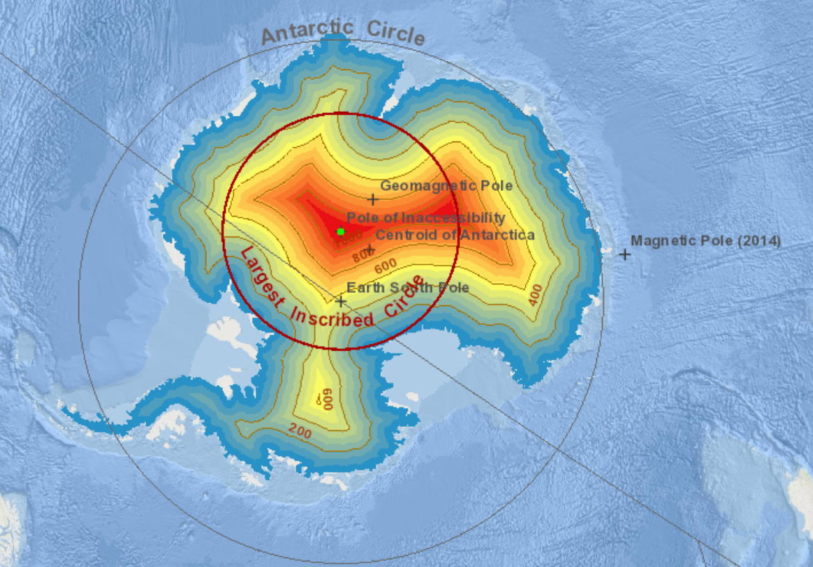
You'll notice that this map of Antarctica is missing the ice shelves, which fill up most of the bays. If the ice shelves are included, then we can draw a larger circle.
As an image processing exercise, I decided to experiment, using the distance transform to measure distances from the coasts, and Julia as the language. Although Julia has now been in development for a decade, it's still a "new kid on the block". But some of its libraries (known as "packages") are remarkably mature and robust. One such is its imaging package Images.
In fact, we need to install and use several packages as well as Images: Colors,
FileIO, ImageView, Plots. These can all be added with Pkg.add("packagename") and brought
into the namespace with using packagename. We also need an image to use, and
for Antarctica I chose this very nice map of the ice surface:
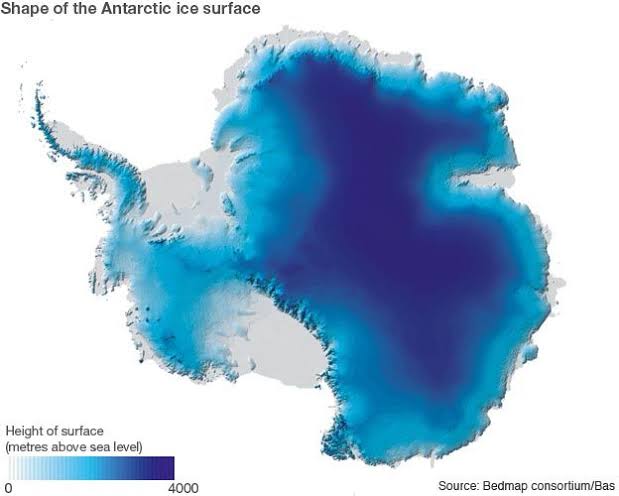
taken from a BBC report. The nice thing about this map is that it shows the ice shelves, so that we can experiment with and without them. We start by reading the image, making it gray-scale, and thresholding it so as to remove the ice-shelves:
julia> ant = load("antarctica.jpg");
julia> G = Gray.(ant);
julia> B = G .> 0.8;
julia> imshow(B)
which produces this:
which as you see has removed the ice shelves. Now we apply the distance transform and find its maximum:
julia> D = distance_transform(feature_transform(B));
julia> findmax(D)
(116.48175822848829, CartesianIndex(214, 350))
This indicates that the largest distance from all edges is about 116, at pixel location (214,350). To show this circle on the image it's easiest to simply plot the image, and then plot the circle on top of it. We'll also plot the centre, as a smaller circle:
julia> plot(ant,aspect_ratio = 1)
julia> x(t) = 214 + 116*cos(t)
julia> x(t) = 350 + 116*sin(t)
julia> xc(t) = 214 + 5*cos(t)
julia> xc(t) = 350 + 5*sin(t)
julia> plot!(y,x,0,2*pi,lw=3,lc="red",leg=false)
julia> plot!(yc,xc,0,2*pi,lw=2,lc="white",leg=false)

This shows the Pole of Inaccessibility in terms of the actual Antarctic continent. However, in practical terms the ice shelves, even though not actually part of the landmass, need to be traversed just the same. To include the ice shelves, we just threshold at a higher value:
julia> B1 = opening(G .> 0.95);
julia> D1 = distance_transform(feature_transform(B1));
julia> findmax(D1)
(160.22796260328596, CartesianIndex(225, 351))
The use of opening in the first line is to fill in any holes in the image: the
distance transform is very sensitive to holes. Then we plot the continent again
with the two circles as above, but using this new centre and radius. This
produces:
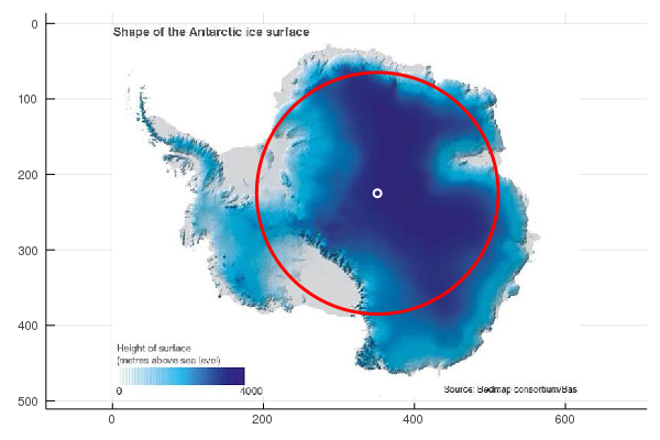
The position of the Pole of Inaccessibility has not in fact changed all that much from the first one.
An interesting sum
I am not an analyst, so I find the sums of infinite series quite mysterious. For example, here are three. The first one is the value of \(\zeta(2)\), very well known, sometimes called the "Basel Problem" and first determined by (of course) Euler: \[ \sum_{n=1}^\infty\frac{1}{n^2}=\frac{\pi^2}{6}. \] Second, subtracting one from the denominator: \[ \sum_{n=2}^\infty\frac{1}{n^2-1}=\frac{3}{4} \] This sum is easily demonstrated by partial fractions: \[ \frac{1}{n^2-1}=\frac{1}{2}\left(\frac{1}{n-1}-\frac{1}{n+1}\right) \] and so the series can be expanded as: \[ \frac{1}{2}\left(\frac{1}{1}-\frac{1}{3}+\frac{1}{2}-\frac{1}{4}+\frac{1}{3}-\frac{1}{5}\cdots\right) \] This is a telescoping series in which every term in the brackets is cancelled except for \(1+1/ 2\), which produces the sum immediately.
Finally, add one to the denominator: \[ \sum_{n=2}^\infty\frac{1}{n^2+1}=\frac{1}{2}(\pi\coth(\pi)-1). \] And this sum is obtained from one of the series representations for \(\coth(z)\):
\[ \coth(z)=\frac{1}{z}+2z\sum_{n=1}^\infty\frac{1}{\pi^2n^2+z^2} \]
(for all \(z\) except for when \(\pi^2n^2+z^2=0\)).
I was looking around for infinite series to give my numerical methods students to test their powers of approximation, and I came across [this beauty](https://www.wolframalpha.com/input/?i=sum+1%2F(n^2%2Bn-1)%2C+n%3D1+to+infinity): \[ \sum_{n=2}^\infty\frac{1}{n^2+n-1}=1+\frac{\pi}{\sqrt{5}}\tan\left(\frac{\sqrt{5}\pi}{2}\right). \] This led me on a mathematical treasure hunt through books and all over the internet, until I had worked it out.
My starting place, after googling "sum quadratic reciprocal" was a very nice and detailed post on stackexchange. This post then referred to a previous one started with the infinite product expression for \(\sin(x)\) and turned it (by taking logarithms and differentiating) into a series for \(\cot(x)\).
However, I want an expression for \(\tan(x)\), which means starting with the infinite product form for \(\sec(x)\), which is:
\[ \sec(x)=\prod_{n=1}^\infty\frac{\pi^2(2n-1)^2}{\pi^2(2n-1)^2-4x^2}. \] Making a substitution simplifies the expression in the product: \[ \sec\left(\frac{\pi x}{2}\right)=\prod_{n=1}^\infty\frac{(2n-1)^2}{(2n-1)^2-x^2}. \] Now take logs of both sides:
\[ \log\left(\sec\left(\frac{\pi x}{2}\right)\right)= \sum_{n=1}^\infty\log\left(\frac{(2n-1)^2}{(2n-1)^2-x^2}\right) \]
and differentiate: \[ \frac{\pi}{2}\tan\left(\frac{\pi x}{2}\right)= \sum_{n=1}^\infty\frac{2x}{(2n-1)^2-x^2}. \] Now we have to somehow equate this new sum on the right with our original sum. So let's go back to it.
First of all, a bit of completing the square produces \[ \frac{1}{n^2+n-1}=\frac{1}{\left(n+\frac{1}{2}\right)^2-\frac{5}{4}}=\frac{4}{(2n+1)^2-5}. \] This means that \[ \sum_{n=1}^\infty\frac{1}{n^2+n-1}=\sum_{n=2}^\infty\frac{4}{(2n-1)^2-5}= \frac{2}{\sqrt{5}}\sum_{n=2}^\infty\frac{2\sqrt{5}}{(2n-1)^2-5}. \] We have changed the index from \(n=1\) to \(n=2\) which allows the rewriting of \(2n+1\) as \(2n-1\). This means we are missing a first term. Comparing the final sum with that for \(\tan(x)\) above, we have \[ \sum_{n=1}^\infty\frac{1}{n^2+n-1}=\frac{2}{\sqrt{5}}\left(\frac{\pi}{2}\tan\left(\frac{\pi \sqrt{5}}{2}\right)-\frac{-\sqrt{5}}{2}\right) \] where the last term is the missing first term: the summand for \(n=1\). Simplifying the right hand side produces \[ \sum_{n=1}^\infty\frac{1}{n^2+n-1}=1+\frac{\pi}{\sqrt{5}}\tan\left(\frac{\sqrt{5}\pi}{2}\right). \] Note that the above series for \(\tan(x)\) can be obtained directly, using a general technique discussed (for example) in that fine old text: "A Course in Modern Analysis", by E. T. Whittaker and G. N. Watson. If \(f(x)\) has only simple poles \(a_n\) with residues \(b_n\), then \[ f(x) = f(0)+\sum_{n=1}^\infty\left(\frac{1}{x-a_n}+\frac{1}{a_n}\right). \] Expressing a function as a series of such reciprocals is known as Mittag-Leffler's theorem and in fact the series for \(\tan(x)\) is given there as one of the examples.
Runge's phenomenon in Geogebra
Runge's phenomenon says roughly that a polynomial through equally spaced points over an interval will wobble a lot near the ends. Runge demonstrated this by fitting polynomials through equally spaced point in the interval \([-1,1]\) on the function \[ \frac{1}{1+25x^2} \] and this function is now known as "Runge's function".
It turns out that Geogebra can illustrate this extremely well.
Equally spaced vertices
Either open up your local version of Geogebra, or go to http://geogebra.org/graphing. In the boxes on the left, enter the following expressions in turn:
- Start by entering Runge's function \[ f(x)=\frac{1}{1+25x^2} \] You should now either zoom in, or use the graph settings tool to display \(x\) between \(-1.5\) and \(1.5\).
- Create a list of \(x\) values: \[ x1 = \frac{\{-5..5\}}{5} \]
- Use those values to create a set of points on the curve: \[ p1 = (x1,f(x1)) \]
- Now create an interpolating polynomial through them: \[ \mathsf{Polynomial}[p1(1)] \]
The resulting graph looks like this:
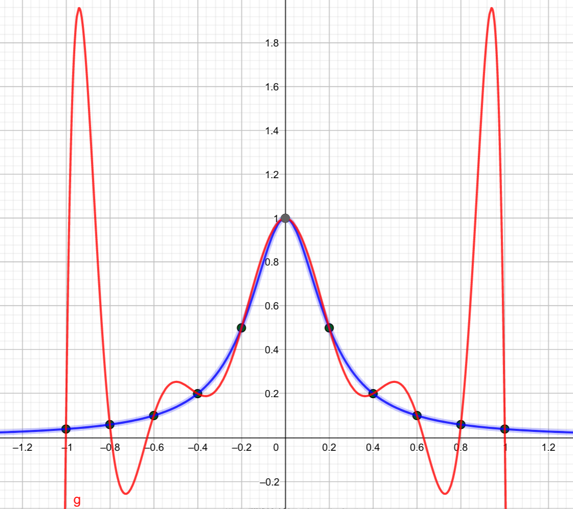
Chebyshev vertices
For the purpose of this post, we'll take the Chebyshev vertices to be those points in the graph whose \(x\) coordinates are given by
\[ x_k = \cos\left(\frac{k\pi}{10}\right) \] for \(k = 0,1,2,\ldots 10\). These values are more clustered at the ends of the interval.
In Geogebra:
- As before, enter the \(x\) values first: \[ x2 = \cos(\frac{\{0..10\}\cdot\pi}{10}) \]
- Then turn them into a sequence of points on the curve \[ p2 = (x2,f(x2)) \]
- Finally create the polynomial through them: \(\mathsf{Polynomial}(p2(1))\).
And this graph looks like this:
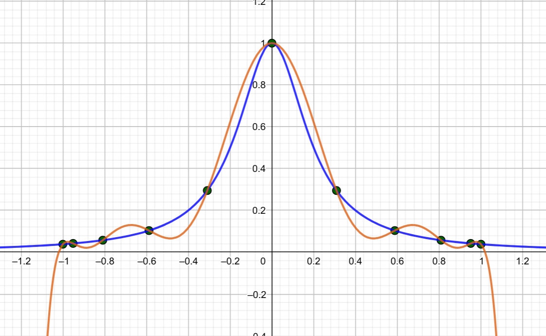
You'll notice how better the second polynomial hugs the curve. The issue is even more pronounced with 21 points, either separated by \(0.1\), or with \(x\) values given by the cosine function again. All we need do is to change the definitions of the \(x\) value sequences \(x1\) and \(x2\) to:
\[ \eqalign{ x1 &= \frac{\{-10..10\}}{10}\\\ x2 &= \cos(\frac{\{0..20\}\pi}{20}) } \]
In fact, you can create a slider \(1\le N \le 20\), say, and then define
\[ \eqalign{ x1 &= \frac{\{-N..N\}}{N}\\\ x2 &= \cos(\frac{\{0..2N\}\pi}{2N}) } \]
and then see how as \(N\) increases, the "Chebyshev" interpolant fits the curve better than the equally spaced interpolant. For \(N=20\), the turning points of the equally spaced polynomial have \(y\) values as high as \(59.78\).
Integration
Using equally spaced values to create an interpolating polynomial and then integrating that polynomial is Newton-Cotes integration. Runge's phenomenon shows why it is better to partition the interval into small sub-intervals and apply a low-order rule to each one. For example, with 20 points on the curve, we would be better applying Simpson's rule to each pair of two sub-intervals, and adding the result. Using a 21-point polynomial is equivalent to a Newton-Cotes rule of order 20, which is far too inaccurate to use.
With our curve \(f(x)\), and our equal-spaced polynomial \(g(x)\), the integrals are
\[ \eqalign{ \int^1_{-1}\frac{1}{1+25x^2},dx&=\frac{2}{5}\arctan(5)\approx 0.5493603067780064\\\ \int^1_{-1}g(x),dx&\approx -5.369910417304622 } \]
However, using the polynomial through the Chebyshev nodes:
\[ \int^1_{-1}h(x)\approx 0.5498082303389538. \]
The absolute errors between the integral values and the exact values are thus (approximately) \(5.92\) and \(0.00045\) respectively.
Integrating an interpolating polynomial through Chebyshev nodes is one way of implementing Clenshaw-Curtis quadrature.
Note that using Simpson's rule on our 21 points produces a value of 0.5485816035037206, which has absolute error of about \(0.0012\).
Fitting the SIR model of disease to data in Python
Introduction and the problem
The SIR model for spread of disease was first proposed in 1927 in a collection of three articles in the Proceedings of the Royal Society by Anderson Gray McKendrick and William Ogilvy Kermack; the resulting theory is known as Kermack–McKendrick theory; now considered a subclass of a more general theory known as compartmental models in epidemiology. The three original articles were republished in 1991, in a special issue of the Bulletin of Mathematical Biology.
The SIR model is so named because it assumes a static population, so no births or deaths, divided into three mutually exclusive classes: those susceptible to the disease; those infected with the disease, and those recovered with immunity from the disease. This model is clearly not applicable to all possible epidemics: there may be births and deaths, people may be re-infected, and so on. More complex models take these and other factors into account.
The SIR model consists of three non-linear ordinary differential equations, parameterized by two growth factors \(\beta\) and \(\gamma\):
\begin{eqnarray*} \frac{dS}{dt}&=&-\frac{\beta IS}{N}\\\ \frac{dI}{dt}&=&\frac{\beta IS}{N}-\gamma I\\\ \frac{dR}{dt}&=&\gamma I \end{eqnarray*}
Here \(N\) is the population, and since each of \(S\), \(I\) and \(R\) represent the number of people in mutually exclusive sets, we should have \(S+I+R=N\). Note that the right hand sides of the equations sum to zero, hence \[ \frac{dS}{dt}+\frac{dI}{dt}+\frac{dR}{dt}=\frac{dN}{dt}=0 \] which indicates that the population is constant.
The problem here is to see if values of \(\beta\) and \(\gamma\) can be found which will provide a close fit to a well-known epidemiological case study: that of influenza in a British boarding school. This was described in a 1978 issue of the British Medical Journal.
This should provide a good test of the SIR model, as it satisfies all of the criteria. In this case there was a total population of 763, and an outbreak of 14 days, with infected numbers as:
| Day: | 1 | 2 | 3 | 4 | 5 | 6 | 7 | 8 | 9 | 10 | 11 | 12 | 13 | 14 | 15 | ||
| Infections: | 1 | 3 | 6 | 25 | 73 | 222 | 294 | 258 | 237 | 191 | 125 | 69 | 27 | 11 | 4 |
Some years ago, on my old (and now taken off line) blog, I explored using Julia for this task, which was managed easily (once I got the hang of Julia syntax). However, that was five years ago, and when I tried to recreate it I found that Julia has changed over the last five years, and my original comments and code no longer worked. So I decided to experiment with Python instead, in which I have more expertise, or at least, experience.
Using Python
- Setup and some initial computation
We start by importing some of the modules and functions we need, and define the data
from the table above:
```python
import matplotlib.pyplot as plt
import numpy as np
from scipy.integrate import solve_ivp
data = [1, 3, 6, 25, 73, 222, 294, 258, 237, 191, 125, 69, 27, 11, 4]
```
Now we enter the SIR system with some (randomly chosen) values of \\(\beta\\) and
\\(\gamma\\), using syntax conformable with the solver `solve_ivp`:
```python
beta,gamma = [0.01,0.1]
def SIR(t,y):
S = y[0]
I = y[1]
R = y[2]
return([-beta*S*I, beta*S*I-gamma*I, gamma*I])
```
We can now solve this system using `solve\_ivp` and plot the results:
```python
sol = solve_ivp(SIR,[0,14],[762,1,0],t_eval=np.arange(0,14.2,0.2))
fig = plt.figure(figsize=(12,4))
plt.plot(sol.t,sol.y[0])
plt.plot(sol.t,sol.y[1])
plt.plot(sol.t,sol.y[2])
plt.plot(np.arange(0,15),data,"k*:")
plt.grid("True")
plt.legend(["Susceptible","Infected","Removed","Original Data"])
```
Note that we have used the `t_eval` argument in our call to `solve_ivp` which
allows us to exactly specify the points at which the solution will be given.
This will allow us to align points in the computed values of \\(I\\) with the
original data.
The output is this plot:
\
There is a nicer plot, with more attention paid to setup and colours,
[here](<https://scipython.com/book/chapter-8-scipy/additional-examples/the-sir-epidemic-model/>).
This use of scipy to solve the SIR equations uses the `odeint` tool. This
works perfectly well, but I believe it is being deprecated in favour of
`solve_ivp`.
- Fitting the data
To find values \\(\beta\\) and \\(\gamma\\) with a better fit to the data, we start by
defining a function which gives the sum of squared differences between the data
points, and the corresponding values of \\(I\\). The problem will then be minimize
that function.
```python
def sumsq(p):
beta, gamma = p
def SIR(t,y):
S = y[0]
I = y[1]
R = y[2]
return([-beta*S*I, beta*S*I-gamma*I, gamma*I])
sol = solve_ivp(SIR,[0,14],[762,1,0],t_eval=np.arange(0,14.2,0.2))
return(sum((sol.y[1][::5]-data)**2))
```
As you see, we have just wrapped the SIR definition and its solution inside a
calling function whose variables are the parameters of the SIR equations.
To minimize this function we need to import another python function first:
```python
from scipy.optimize import minimize
msol = minimize(sumsq,[0.001,1],method='Nelder-Mead')
msol.x
```
with output:
```python
array([0.00218035, 0.44553886])
```
To see if this does provide a better fit, we can simply run the solver with
these values, and plot them, as we did at the beginning:
```python
beta,gamma = msol.x
def SIR(t,y):
S = y[0]
I = y[1]
R = y[2]
return([-beta*S*I, beta*S*I-gamma*I, gamma*I])
```
```python
sol = solve_ivp(SIR,[0,14],[762,1,0],t_eval=np.arange(0,14.2,0.2))
```
```python
fig = plt.figure(figsize=(10,4))
plt.plot(sol.t,sol.y[0],"b-")
plt.plot(sol.t,sol.y[1],"r-")
plt.plot(sol.t,sol.y[2],"g-")
plt.plot(np.arange(0,15),data,"k*:")
plt.legend(["Susceptible","Infected","Removed","Original Data"])
```
with output:
\
and as you see, a remarkably close fit!
Mapping voting gains between elections
So this goes back quite some time to the recent Australian Federal election on May 18. In my own electorate (known formally as a "Division") of Cooper, the Greens, who until recently had been showing signs of winning the seat, were pretty well trounced by Labor.
- Some background asides
First, "Labor" as in "Australian Labor Party" is spelled the
American way; that is, without a "u", even though "labour" meaning work, is so
spelled in Australian English.  This is because much of Australia's pre-federal
political history has a large American influence; indeed one of the loudest
political voices in the 19th century was [King
O'Malley](<https://en.wikipedia.org/wiki/King%5FO%27Malley>) who was born in 1858 in
Kansas, and didn't come to Australia until he was about 30. He was responsible,
amongst other things, for selecting the site for Canberra (the nation's capital)
and in selecting Walter Burley Griffin as its architect.  As well, the
Australian Constitution shows a large American influence; the constitutions of
both countries bear a remarkably close resemblance, and Australia's parliament
is modelled on that of the United States Congress.

Second, my electorate was formerly known as "Batman" after [John
Batman](<https://en.wikipedia.org/wiki/John%5FBatman>), the supposed founder of
Melbourne.  However, Batman was known in his lifetime as a contemptible figure,
and the historical record well bears out the description of him as "the vilest
man I have ever known".  He was responsible for the slaughter of indigenous
peoples, and his so called "treaty" with the people of the Kulin Nation in
exchange for land on what would would become Melbourne is considered invalid.
In respect for the local peoples ("who have never ceded sovereignty"), the
electorate was renamed last year in honour of
[William Cooper](<https://en.wikipedia.org/wiki/William%5FCooper%5F(Aboriginal%5FAustralian)>), a
Yorta Yorta elder, a tireless activist for Aboriginal rights, and the only
individual in the world to lodge a formal protest to a German embassy on the
occasion of Kristallnacht.
- Back to mapping
All I wanted to do was to map the size of Labor's gains (over the Greens)
between the last election in 2016 and this one, at
each polling booth in the electorate. For this I used the following Python
packages: [matplotlib](<https://matplotlib.org/>),
[pandas](<https://pandas.pydata.org/>), [geopandas](<http://geopandas.org/>),
[numpy](<https://numpy.org/>),
[cartopy](<https://scitools.org.uk/cartopy/docs/latest/>). The nice thing about
Python, for me at least, is the ease of prototyping, and the availability of
packages for just about everything. Indeed, for an amateur programmer like
myself, one of the biggest difficulties is finding the right package for the
job. There's a score or more for GIS alone.
All information about the election can be downloaded from the [Australian
Electorial Commission
tallyroom](<https://tallyroom.aec.gov.au/HouseDefault-24310.htm>). And the GIS
information can be obtained also from the
[AES](<https://www.aec.gov.au/Electorates/gis/gis%5Fdatadownload.htm>). The
Victorian [shapefile](<https://en.wikipedia.org/wiki/Shapefile>) needs to be
unzipped before using.
Then the map set-up looks like this:
```python
shp = gpd.read_file('VicMaps/E_AUGFN3_region.shp')
cooper = shp.loc[shp['Elect_div']=='Cooper']
bounds = cooper.geometry.bounds
bg = bounds.values[0] # latitude, longitude of extent of region
pad = 0.01 # padding for display
extent = [bg[0]-pad,bg[2]+pad,bg[1]-pad,bg[3]+pad]
```
The idea of the padding is simply to ensure that the map, once displayed,
extends beyond the area of the electorate. The units are degrees of latitude
and longitude. In Melbourne, at about 37.8 degrees south, 0.01 degrees latitude
corresponds to about 1.11km, and 0.01 degrees longitude corresponds to about 0.88km.
Now we need to determine the percentage of votes to Labor (on a two-party
preferred computation) which again involves reading material from the AEC site.
I downloaded it first, but it could also be read directly from the site into
pandas.
```python
# Get all votes by polling booths in Cooper for 2019
b19 = pd.read_csv('Elections/TCPByCandidateByPollingPlaceVIC-2019.csv') # b19 = booths, 2019
v19 = b19.loc[b19.DivisionNm=='Cooper'] # v19 = Cooper Booths, 2019
v19 = v19[['PollingPlace','PartyAb','OrdinaryVotes']]
v19r = v19.loc[v19.PartyAb=='GRN']
v19k = v19.loc[v19.PartyAb=='ALP']
v19c = v19r.merge(v19k,left_on='PollingPlace',right_on='PollingPlace') # Complete votes
v19c['Percent_x'] = (v19c['OrdinaryVotes_x']*100/(v19c['OrdinaryVotes_x']+v19c['OrdinaryVotes_y'])).round(2)
v19c['Percent_y'] = (v19c['OrdinaryVotes_y']*100/(v19c['OrdinaryVotes_x']+v19c['OrdinaryVotes_y'])).round(2)
v19c = v19c.dropna()
# note: suffix -x is GRN; suffix _y is ALP
```
The next step is to determine the positions of all polling places. For
simplification, I'm only interested in places used in both this most recent
election, and the previous federal election in 2016:
```python
v16 = pd.read_csv('Elections/Batman2016_TCP.csv')
v_both = v16.merge(v19c,right_on='PollingPlace',left_on='Booth')
c19 = pd.read_csv('Elections/Cooper_PollingPlaces.csv')
c19 = c19.drop(44).reset_index() # Drop Special Hospital, which has index 44
v_all=v_both.merge(c19,left_on='PollingPlace',right_on='PollingPlaceNm')
lats = np.array(v_all['Latitude'])
longs = np.array(v_all['Longitude'])
booths = np.array(v_all['PollingPlaceNm'])
diffs = np.array(v_all['Percent_y']-v_all['ALP percent']) # change in ALP percentage
```
Having now got the boundary of the electorate, the positions of each polling
booth, the percentage change in votes for Labor, the map can now be created and
displayed:
```python
fig = plt.figure(figsize = (16,16))
tiler = GoogleTiles()
ax = plt.axes(projection=tiler.crs)
ax.set_extent(extent)
ax.add_image(tiler, 13, interpolation='hanning')
ax.add_geometries(cooper.geometry,crs=ccrs.PlateCarree(),facecolor='none',edgecolor='k',linewidth=2)
for i in range(34):
if diffs[i]>0:
ax.plot(longs[i],lats[i],marker='o',markersize=diffs[i],markerfacecolor='r',transform=ccrs.Geodetic())
else:
ax.plot(longs[i],lats[i],marker='o',markersize=-diffs[i],markerfacecolor='g',transform=ccrs.Geodetic())
plt.show()
```
I found by trial and error that Hanning interpolation seemed to give the best
results.
\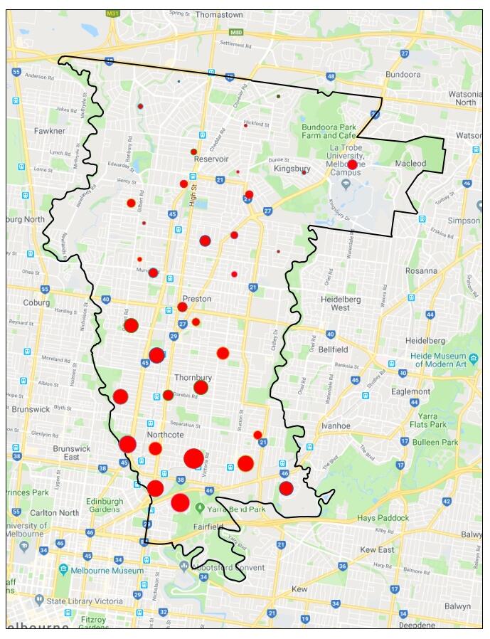
So this image shows not the size of Labor's _vote_, but the size of Labor's
_gain_ since the previous election. The larger gains are in the southern part of
the electorate: the northern part has always been more Labor friendly, and so the
gains were smaller there.
Educational disciplines: size against market growth
Here is an interactive version of this diagram:
[!APF Figure 4](/APF_figure_4.png)
(click on the image to show a larger version.)
Tschirnhausen transformations and the quartic
Here we show how a Tschirnhausen transformation can be used to solve a quartic equation. The steps are:
-
Ensure the quartic is missing the cubic term, and its initial coefficient is 1. We can do this by first dividing by the initial coefficient to obtain an equation \[ x^4+b_3x^3+b_2x^2+b_1x+b_0=0 \] and then replace the variable \(x\) with \(y=x-b_3/ 4\). This will produce a monic quartic equation missing the cubic term.
We can thus take \[ x^4+bx^2+cx+d=0 \] as a completely general formulation of the quartic equation.
-
Now apply the Tschirnhausen transformation \[ y = x^2+rx+s \] using the resultant, which will produce a quartic equation in \(y\).
-
Chose \(r\) and \(s\) so that the coefficients of the linear and cubic terms are zero. This will require solving a cubic equation.
-
Substitute those \(r,s\) values into the resultant, which will produce a biquadratic equation in \(y\): \[ y^4+Ay^2+B=0. \] This can be readily solved as it's a quadratic in \(y^2\). Finally, for each value of \(y\), and using the \(r,s\) values, solve \[ x^2+rx+s-y=0. \] This will in fact produce eight values, of which four are the solution to the original quartic.
An example
Consider the equation \[ x^4-94x^2-480x-671=0 \] which has solutions
\begin{align*} x &= -2 , \sqrt{5} \pm \sqrt{3} \sqrt{9 -4, \sqrt{5}},\\\ x &= 2 , \sqrt{5} \pm \sqrt{3} \sqrt{9 + 4 , \sqrt{5}} \end{align*}
Note that these relatively nice solutions arise from the polynomial being factorizable in the number field \(\mathbb{Q}[\sqrt{5}]\). We can show this using Sagemath:
N.<a> = NumberField(x^2-5)
K.<x> = N[]
factor(x^4 - 94*x^2 - 480*x - 671)
\[ (x^{2} - 4 a x - 12 a - 7) \cdot (x^{2} + 4 a x + 12 a - 7) \]
We shall continue to use Sagemath to perform all the dirty work; here's how this solution works:
var('x,y,r,s')
qx = x^4 - 94*x^2 - 480*x - 671
res = qx.resultant(y-x^2-r*x-s,x).poly(y)
We now want to find the values of \(r\) and \(s\) to eliminate the linear and cubic terms. The cubic term is easy:
res.coefficient(y,3)
\[ -4s-188 \] and so
s_sol = solve(res.coefficient(y,3),s,solution_dict=True)
and we can substitute this into the linear coefficient:
res.coefficient(y,1).subs(s_sol[0]).factor()
\[ -480(r+10)(r+8)(r+6). \] In general the coefficient would not be as neatly factorizable as this, but we can still find the values of \(r\):
r_sol = solve(res.coefficient(y,1).subs(s_sol[0]),r,solution_dict=True)
We can choose any value we like; here let's choose the first value and substitute it into the resultant from above, first creating a dictionary to hold the \(r\) and \(s\) values:
rs = s_sol[0].copy()
rs.update(r_sol[0])
rs
\[ \lbrace s:-47,r:-8\rbrace \]
res.subs(rs)
\[ y^4-256y^2+1024 \]
y_sol = solve(res.subs(rs),y,solution_dict=True)
This will produce four values of \(y\), and for each one we solve the equation \[ x^2+rx+s-y=0 \] for \(x\):
for ys in ysol:
    display(solve((x^2+r*x+s-y).subs(rs).subs(ys),x))
\begin{align*} x &= -\sqrt{-4 , \sqrt{2 , \sqrt{15} + 8} + 63} + 4,& x &= \sqrt{-4 , \sqrt{2 , \sqrt{15} + 8} + 63} + 4\\\ x &= -\sqrt{4 , \sqrt{2 , \sqrt{15} + 8} + 63} + 4,& x& = \sqrt{4 ,\sqrt{2 , \sqrt{15} + 8} + 63} + 4\\\ x& = -\sqrt{-4 , \sqrt{-2 , \sqrt{15} + 8} + 63} + 4,& x& = \sqrt{-4 ,\sqrt{-2 , \sqrt{15} + 8} + 63} + 4\\\ x& = -\sqrt{4 , \sqrt{-2 , \sqrt{15} + 8} + 63} + 4,& x& = \sqrt{4 , \sqrt{-2 , \sqrt{15} + 8} + 63} + 4 \end{align*}
We can check these values to see which ones are actually correct. But to experiment, we can determine the minimal polynomial of each value given:
for ys in ysol:
    s1 = solve((x^2+r*x+s-y).subs(rs).subs(ys),x,solution_dict=True)
    ql = [QQbar(z[x]).minpoly() for z in s1]
    display(ql)
\begin{align*} &x^{4} - 94 x^{2} - 480 x - 671,&& x^{4} - 32 x^{3} + 290 x^{2} - 64 x - 6431&\\\ &x^{4} - 94 x^{2} - 480 x - 671,&& x^{4} - 32 x^{3} + 290 x^{2} - 64 x - 6431&\\\ &x^{4} - 32 x^{3} + 290 x^{2} - 64 x - 6431,&& x^{4} - 94 x^{2} - 480 x - 671&\\\ &x^{4} - 94 x^{2} - 480 x - 671,&& x^{4} - 32 x^{3} + 290 x^{2} - 64 x - 6431& \end{align*}
Half of these are the original equation we tried to solve. And the others?
qx.subs(x=8-x).expand()
\[ x^{4} - 32 x^{3} + 290 x^{2} - 64 x - 6431 \] This is in fact what we should expect, from solving the equation \[ x^2+rx+s-y=0 \] If the roots are \(x_1\) and \(x_2\), then by Vieta's formulas \(x_1+x_2=-(-r)=r\).
Further comments
The trouble with this method is that it only works nicely on some equations. In general, the snarls of square, cube, and fourth roots become unwieldy very quickly. For example, consider the equation \[ x^4+6x^2-60x+36=0 \] which according to Cardan in Ars Magna (Chapter XXXIX, Problem V) was first solved by Ferrari.
Taking the resultant with \(y-x^2-rx-s\) as a polynomial on \(y\), we find that the coefficient of \(y^3\) is \(-4s+12\), and so \(s=3\). Substituting this in the linear coefficient, we obtain this cubic in \(r\): \[ 5r^3-9r^2-60r+300=0. \] The simplest (real) solution is: \[ r = \frac{1}{5} , {\left(50 , \sqrt{3767} - 3273\right)}^{\frac{1}{3}} + \frac{109}{5 , {\left(50 , \sqrt{3767} - 3273\right)}^{\frac{1}{3}}} + \frac{3}{5} \] Substituting these values of \(r\) and \(s\) into the resultant, we obtain the equation \[ y^4+c_2y^2+c_0=0 \] with \[ c_2=\frac{6 , {\left({\left(50 , \sqrt{3767} - 3273\right)}^{\frac{2}{3}} {\left(50 , \sqrt{3767} - 18969\right)} - {\left(7200 , \sqrt{3767} - 483193\right)} {\left(50 , \sqrt{3767} - 3273\right)}^{\frac{1}{3}} + 100 , \sqrt{3767} - 6546\right)}}{25 , {\left(50 , \sqrt{3767} - 3273\right)}} \] and \[ c_0=\frac{27\left(% \begin{array}{l} 2,(14353657451700 , \sqrt{3767} - 880869586608887), (50 , \sqrt{3767} - 3273)^{\frac{2}{3}}\\\ \quad+109541 , (2077754350 , \sqrt{3767} - 127532539917) (50 , \sqrt{3767} - 3273)^{\frac{1}{3}}\quad{}\\\ \hspace{18ex} - 5262543802068000 , \sqrt{3767} + 322980491997672634 \end{array}% \right)} {625 , {\left(2077754350 , \sqrt{3767} - 127532539917\right)} {\left(50 , \sqrt{3767} - 3273\right)}^{\frac{1}{3}}} \] Impressed?
Right, so we solve the equation for \(y\), to obtain \[ y=\pm\sqrt{-\frac{1}{2}c_2\pm\frac{1}{2}\sqrt{c_2^2-4c_0}}. \] For each of those values of \(y\), we solve the equation \[ x^2+rx+s-y=0 \] to obtain (for example) \[ x= = -\frac{1}{2} , r \pm \frac{1}{2} , \sqrt{r^{2} - 4 , s + 4 , \sqrt{-\frac{1}{2} , c_{2} + \frac{1}{2} , \sqrt{c_{2}^{2} - 4 , c_{0}}}} \] With \(r\) being the solution of a cubic equation, and \(c_0\), \(c_2\) being the appalling expressions above, you can see that this solution, while "true" in a logical sense, is hardly useful or enlightening.
Cardan again: "So progresses arithmetic subtlety, the end of which, it is said, is as refined as it is useless."
Tschirnhausen's solution of the cubic
A general cubic polynomial has the form \[ ax^3+bx^2+cx+d \] but a general cubic equation can have the form \[ x^3+ax^2+bx+c=0. \] We can always divide through by the coefficient of \(x^3\) (assuming it to be non-zero) to obtain a monic equation; that is, with leading coefficient of 1. We can now remove the \(x^2\) term by replacing \(x\) with \(y-a/3\): \[ \left(y-\frac{a}{3}\right)^{\negmedspace 3}+a\left(y-\frac{a}{3}\right)^{\negmedspace 2} +b\left(y-\frac{a}{3}\right)+c=0. \] Expanding and simplifying produces \[ y^3+\left(b-\frac{a^2}{3}\right)y+\frac{2}{27}a^3-\frac{1}{3}ab+c=0. \] In fact this can be simplified by writing the initial equation as \[ x^3+3ax^2+bx+c=0 \] and then substituting \(x=y-a\) to obtain \[ y^3+(b-3a^2)y+(2a^3-ab+c)=0. \] This means that in fact an equation of the form \[ y^3+Ay+B=0 \] is a completely general form of the cubic equation. Such a form of a cubic equation, missing the quadratic term, is known as a depressed cubic.
We could go even further by substituting \[ y=z\sqrt{A} \] to obtain
\[ A^{3/ 2}z^3+A\sqrt{A}z+B=0 \]
and dividing through by \(A^{3/ 2}\) to produce
\[ z^3+z+BA^{-3/ 2}=0. \]
This means that
\[ z^3+z+W=0 \]
is also a perfectly general form for the cubic equation.
Cardan's method
Although this is named for Gerolamo Cardano (1501-1576), the method was in fact discovered by Niccolò Fontana (1500-1557), known as Tartaglia ("the stammerer") on account of a injury obtained when a soldier slashed his face when he was a boy. In the days before peer review and formal dissemination of ideas, any new mathematics was closely guarded: mathematicians would have public tests of skill, and a new solution method was invaluable. After assuring Tartaglia that his new method was safe with him, Cardan then proceeded to publish it as his own in his magisterial Ars Magna in 1545. A fascinating account of the mix of Cardan, Tartaglia, and several other egotistic mathematicians of the time, can be read here.
Cardan's method solves the equation \[ x^3-3ax-2b=0 \] noting from above that this is a perfectly general form for the cubic, and where we have introduced factors of \(-3\) and \(-2\) to eliminate fractions later on. We start by assuming that the solution will have the form \[ x=p^{1/ 3}+q^{1/ 3} \] and so \[ x^3=(p^{1/ 3}+q^{1/ 3})^3=p+3p^{2/ 3}q^{1/ 3}+3p^{1/ 3}q^{2/ 3}+q. \] This last can be written as \[ p+q+3p^{1/ 3}q^{1/ 3}(p^{1/ 3}+q^{1/ 3}). \] We can thus write \[ x^3=3p^{1/ 3}q^{1/ 3}x+p+q \] and comparing with the initial cubic equation we have \[ 3p^{1/ 3}q^{1/ 3}=3a,\quad p+q=2b. \] These can be written as \[ pq=a^3,\quad p+q=2b \] for which the solutions are \[ p,q=b\pm\sqrt{b^2-a^3} \] and so \[ x = (b+\sqrt{b^2-a^3})^{1/ 3}+(b-\sqrt{b^2-a^3})^{1/ 3}. \] This can be written in various different ways.
For example, \[ x^3-6x-6=0 \] for which \(a=2\) and \(b=3\). Here \(b^2-a^3=1\) and so one solution is \[ x=4^{1/ 3}+2^{1/ 3}. \] Given that a cubic must have three solutions, the other two are \[ \omega p^{1/ 3}+\omega^2 q^{1/ 3},\quad \omega^2 p^{1/ 3}+\omega q^{1/ 3} \] where \(\omega\) is a cube root of 1, for example \[ \omega=\frac{1}{2}+i\frac{\sqrt{3}}{2}. \]
And so to Tschirnhausen
At the beginning we eliminated the \(x^2\) terms from a cubic equation by a linear substitution \(x=y-a/3\) or \(y=x+a/3\). Writing in the year 1680, the German mathematician Ehrenfried Walther von Tschirnhausen (1651-1708) began experimenting with more general polynomial substitutions, believing that it would be possible to eliminate other terms at the same time. Such substitutions are now known as Tschirnhausen transformations and of course the modern general approach places them squarely within field theory.
Tschirnhausen was only partially correct: it is indeed possible to remove some terms from a polynomial equation, and in 1858 the English mathematician George Jerrard (1804-1863) showed that it was possible to remove the terms of degree \(n-1\), \(n-2\) and \(n-3\) from a polynomial of degree \(n\). In particular, the general quintic equation can be reduced to \[ x^5+px+q=0 \] which is known as the Bring-Jerrard form; also honouring Jerrard's predecessor, the Swedish mathematician Erland Bring (1736-1798). Note that Jerrard was quite well aware of the work of Ruffini, Abel and Galois in proving the general unsolvability by radicals of the quintic equation.
Neither Bring nor Tschirnhausen had the advantage of this knowledge, and both were working towards a general solution of the quintic.
Happily, Tschirnhausen's work is available in an English translation, published in the ACM SIGSAM Bulletin by R. F. Green in 2003. For further delight, Jerrard's text, with the splendidly formal English title "An Essay on the Resolution of Equations", is also available online.
After that history lesson, let's explore how to remove both the quadratic and linear terms from a cubic equation using Tschirnhausen's method, and also using SageMath to do the heavy algebraic work. There is in fact nothing particularly conceptually difficult, but the algebra is quite messy and fiddly.
We start with a depressed cubic equation \[ x^3+3ax+2b=0 \] and we will use the Tschirnhausen transformation \[ y=x^2+rx+s. \]
This can be done by hand of course, using a somewhat fiddly argument, but for us the best approach is to compute the resultant of the two polynomials, which is a polynomial expression equal to zero if the two polynomials have a common root. The resultant can be computed as the determinant of the Sylvester matrix (named for its discoverer); but we can simply use SageMath:
var('a,b,c,x,y,r,s')
cb = x^3 + 3*a*x + 2*b
res = cb.resultant(y-x^2-r*x-s,x).poly(y)
res
\[ \displaylines{ y^3+3(2a-s)y^{2}+3(ar^{2}+3a^{2}+2r-4as+s^{2})y\\\ {\ }\mspace4em -4b^{2}+2br^{3}-3ar^{2}s+6abr-9a^{2}s-6brs+6as^{2}-s^{3} } \]
Now we find values of \(r\) and \(s\) for which the coefficients of \(y^2\) and \(y\) will be zero:
sol = solve([res.coefficient(y,1),res.coefficient(y,2)],[r,s],solution_dict=True)
sol
\[ \left[\left\lbrace s : 2 , a, r : -\frac{b + \sqrt{a^{3} + b^{2}}}{a}\right\rbrace, \left\lbrace s : 2 , a, r : -\frac{b - \sqrt{a^{3} + b^{2}}}{a}\right\rbrace\right] \]
We can now substitute say the second solution into the resultant from above, which should produce an expression of the form \(y^3+A\):
cby = res.subs(sol[1]).canonicalize_radical().poly(y)
cby
\[ y^3-8 , a^{3} - 16 , b^{2} + 8 , \sqrt{a^{3} + b^{2}} b - \frac{8 , b^{4}}{a^{3}} + \frac{8 , \sqrt{a^{3} + b^{2}} b^{3}}{a^{3}} \] We can simply take the cube root of the constant term as our solution:
sol_y = solve(cby,y,solution_dict=True)
sol_y[2]
\[ \left\lbrace y : \frac{2 , {\left(a^{6} + 2 , a^{3} b^{2} - \sqrt{a^{3} + b^{2}} a^{3} b + b^{4} - \sqrt{a^{3} + b^{2}} b^{3}\right)}^{\frac{1}{3}}}{a}\right\rbrace \]
Now we solve the equation \(y=x^2+rx+s\) using the values \(r\) and \(s\) from above, and the value of \(y\) just obtained:
eq = x^2+r*x+s-y
eqrs = eq.subs(sol[1])
eqx = eqrs.subs(sol_y[2])
solx =  solve(eqx,x,solution_dict=True)
solx[0]
\[ \left\lbrace x : \frac{b - \sqrt{a^{3} + b^{2}} - \sqrt{-7 , a^{3} + 2 , b^{2} - 2 , \sqrt{a^{3} + b^{2}} b + 8 , {\left(a^{6} + 2 , a^{3} b^{2} + b^{4} - {\left(a^{3} b + b^{3}\right)} \sqrt{a^{3} + b^{2}}\right)}^{\frac{1}{3}} a}}{2 , a}\right\rbrace \]
A equation, of err... rare beauty, or if not beauty, then something else. It certainly lacks the elegant simplicity of Cardan's solution. On the other hand, the method can be applied to quartic (and quintic) equations, which Cardan's solution can't.
Finally, let's test this formula, again on the equation \(x^3-6x-6=0\), for which \(a=-2\) and \(b=-3\):
xs = solx[0][x].subs({a:-2, b:-3})
xs
\[ \frac{1}{4} , \sqrt{-16 \cdot 4^{\frac{1}{3}} + 80} + 1 \]
This can clearly be simplified to
\[ 1+\sqrt{5-4^{1/ 3}} \] It certainly looks different from Cardan's result, but watch this:
xt = QQbar(xs)
xt.radical_expression()
\[ \frac{1}{2}4^{2/ 3}+4^{1/ 3} \]
which is Cardan's result, only very slightly rewritten. And finally:
xt.minpoly()
\[ x^3-6x-6 \]
Colonial massacres, 1794 to 1928
The date January 26 is one of immense current debate in Australia. Officially it's the date of Australia Day, which supposedly celebrates the founding of Australia. To Aboriginal peoples it is a day of deep mourning and sadness, as the date commemorates over two centuries of oppression, bloodshed, and dispossession. To them and their many supporters, January 26 is Invasion Day.
The date commemorates the landing in 1788 of Arthur Phillip, in charge of the First Fleet and the first Governor of the colony of New South Wales.
The trouble is that "Australia" means two things: the island continent, and the country. The country didn't exist until Federation on January 1, 1901; before which time the land since 1788 was subdivided into independent colonies. Many people believe that Australia Day would be better moved to January 1; the trouble with that is that it's already a public holiday, and apparently you can't have a national day that doesn't have its own public holiday. And many other dates have been proposed.
My own preferred date is June 3; this is the date of the High Court "Mabo" decision in 1992 which formally recognized native title and rejected the doctrine of terra nullius under which the British invaded.
That the continent was invaded rather than settled is well established: all serious historians take this view, and it can be backed up with legal arguments. The Aboriginal peoples, numbering maybe close to a million in 1788, had mastered the difficult continent and all of its many ecosystems, and had done so for around 80,000 years. Aboriginal culture is the oldest continually maintained culture on the planet, and by an enormous margin.
Arthur Phillip did in fact arrive with formal instructions to create "amity" with the "natives" and indeed to live in "kindness" with them, but this soon went downhill. Although Phillip himself seems to have been a man of rare understanding for his time (when speared in the shoulder, for example, he refused to let his soldiers retaliate), he was no match for the many convicts and soldiers under his rule. When he retired back to England in 1792 the colony was ruled by a series of weak and ineffective governors, and in particular by the military, culminating in the governorship of Lachlan Macquarie who is seen as a mass murderer of Aboriginal peoples, although the evidence is not clear-cut. What is clear is that mass murders of Aboriginal peoples were common and indiscriminate, and often with appalling cruelty. On many occasions large groups were poisoned with strychnine: this works by affecting the nerves which control muscle movement, so that the body goes into agonizing spasms resulting in death by asphyxiation. Strychnine is considered by toxicologists to be one of the most painful acting of all poisons. Even though Macquarie himself ordered retribution only after "resistance"; groups considered harmless, or consisting only of old men, women and children, were brutally murdered.
People were routinely killed by gunfire, or by being hacked to death; there is at least one report of a crying baby - the only survivor of a massacre - being thrown onto the fire made to burn the victims.
Many more died of disease: smallpox and tuberculosis were responsible for deaths of over 50% of Aboriginal peoples. Their numbers today are thus tiny, and as in the past they are still marginalized.
Only recently has this harrowing part of Australia's past been formally researched; the casual nature of the massacres meant that many were not recorded, and it has taken a great deal of time and work to uncover their details. This work has been headed by Professor Lyndall Ryan at the University of Newcastle. The painstaking and careful work by her team has unearthed much detail, and their results are available at their site Colonial Frontier Massacres in Central and Eastern Australia 1788-1930
As a January 26 exercise I decided to rework one of their maps, producing a single map which would show the sites of massacres by markers whose size is proportional to the number of people killed. This turned out to be quite easy using Python and its folium library, but naturally it took me a long time to get it right.
I started by downloading the timeline from the Newcastle site as a csv file, and going through each massacre adding its location. The project historians point out that the locations are deliberately vague. Sometimes this is because the vagueness of the historical record; but also (from the Introduction):
In order to protect the sites from desecration, and respect for the wishes of Aboriginal communities to observe the site as a place of mourning, the points have been made purposefully imprecise by rounding coordinates to 3 digits, meaning the point is precise only to around 250m.
Given the database, the Python commands were:
import folium
import pandas as pd

mass = pd.read_csv('massacres.csv')

a = folium.Map(location=[-27,134],width=1000, height=1000,tiles='OpenStreetMap',zoom_start=4.5)

for i in range(0,len(mass)):
   number_killed = mass.iloc[i]['Estimated Aboriginal People Killed']
   folium.Circle(
      location=[float(mass.iloc[i]['Lat']), float(mass.iloc[i]['Long'])],
      tooltip=mass.iloc[i]['Location']+': '+str(number_killed),
      radius=int(number_killed)*150,
      color='goldenrod',
      fill=True,
      fill_color='gold'
   ).add_to(a)

a.save("massacres.html")
The result is shown below. You can zoom in and out, and hovering over a massacre site will produce the location and number of people murdered.
The research is ongoing and this data is incomplete
The data was extracted from: Ryan, Lyndall; Richards, Jonathan; Pascoe, William; Debenham, Jennifer; Anders, Robert J; Brown, Mark; Smith, Robyn; Price, Daniel; Newley, Jack Colonial Frontier Massacres in Eastern Australia 1788 – 1872, v2.0 Newcastle: University of Newcastle, 2017, http://hdl.handle.net/1959.13/1340762 (accessed 08/02/2019). This project has been funded by the Australian Research Council (ARC).
Note finally that Professor Ryan and team have defined a massacre to be a killing of at least six people. Thus we can assume there are many other killings of five or less people which are not yet properly documented, or more likely shall never been known. A shameful history indeed.
Vote counting in the Australian Senate
Recently we have seen senators behaving in ways that seem stupid, or contrary to accepted public opinion. And then people will start jumping up and down and complaining that such a senator only got a tiny number of first preference votes. One commentator said that one senator, with 19 first preference votes, "couldn’t muster more than 19 members of his extended family to vote for him". This displays an ignorance of how senate counting works. In fact first preference votes are almost completely irrelevant; or at least, far less relevant than they are in the lower house.
Senate counting works on a proportional system, where multiple candidates are elected from the same group of ballots. This is different from the lower house (the House of Representatives federally) where only one person is elected. For the lower house, first preference votes are indeed much more important. As for the lower house, senate voting is preferential: voters number their preferred candidates starting with 1 for their most preferred, and so on (but see below).
A full explanation is given by the Australian Electoral Commission on their Senate Counting page; this blog post will run through a very simple example to demonstrate how a senator can be elected with a tiny number of first preference votes.
An aside on micro parties and voting
One problem in Australia is the proliferation of micro parties, many of which hold racist, anti-immigration, or hard-line religious views, or who in some other ways represent only a tiny minority of the electorate. The problem is just as bad at State level; in my own state of Victoria we have the Shooters, Fishers and Farmers Party, the Aussie Battlers Party, and the Transport Matters Party (who represent taxi drivers) to name but three. This has the affect that the number of candidates standing for senate election has become huge, and the senate ballot papers absurdly unwieldy:

Initially the law required voters to number every box starting from 1: on a large paper this would mean numbering carefully from 1 up to at least 96 in one recent election. To save this trouble (and most Australian voters are nothing if not lazy), "above the line voting" was introduced. This gave voters the option to put just a single "1" in the box representing the party of choice: you will see from the image above that the ballot paper is divided: the columns represent all the parties; the boxes below the line represent all the candidates from that party, and the single box above just the party name. Here is a close up of a NSW senate ballot:

Almost all voters willingly took advantage of that and voted above the line. The trouble is then that voters have no control over where their preferences go: that is handled by the parties themselves. By law, all parties must make their preferences available before the election, and they are published on the site of the relevant Electoral Commission. But the only people who carefully check this site and the party's preferences are the sort of people who would carefully number each box below the line anyway. Most people don't care enough to be bothered.
This enables all the micro-parties to make "preference deals"; in effect they act as one large bloc, ensuring that at least some of them get a senate seat. This has been handled by a so-called "preference whisperer".
The current system in the state of Victoria has been to encourage voting below the line by allowing, instead of all boxes to be numbered, at least six. And there are strong calls for voting above the line to be abolished.
A simple example
To show how senate counting works, we suppose an electorate of 100 people, and three senators to be elected from five candidates. We also suppose that every ballot paper has been numbered from 1 to 5 indicating each voter's preferences.
Before the counting begins we need to determine the number of votes each candidate must amass to be elected: this is chosen as the smallest number of votes for which no more candidates can be elected. If there are \(n\) formal votes cast, and \(k\) senators to be elected, that number is clearly
\[\left\lfloor\frac{n}{k+1}\right\rfloor + 1.\]
This value is known as the Droop quota. In our example, this quota is
\[ \left\lfloor\frac{100}{3+1}\right\rfloor +1 = 26. \]
You can see that it is not possible for four candidates to obtain this value.
Suppose that the ballots are distributed as follows, where the numbers under the candidates indicate the preferences cast:
| Number of votes | A | B | C | D | E |
|---|---|---|---|---|---|
| 20 | 1 | 2 | 3 | 4 | 5 |
| 20 | 1 | 5 | 4 | 3 | 2 |
| 40 | 2 | 1 | 5 | 4 | 3 |
| 5 | 2 | 3 | 5 | 1 | 4 |
| 4 | 4 | 3 | 1 | 2 | 5 |
| 1 | 2 | 3 | 4 | 5 | 1 |
Counting first preferences produces:
| Candidate | First Prefs |
|---|---|
| A | 40 |
| B | 40 |
| C | 4 |
| D | 5 |
| E | 1 |
The first step in the counting is to determine if any candidate has amassed first preference votes equal to or greater than the Droop quota. In the example just given, both A and B have 40 first preferences each, so they are both elected.
Since only 26 votes are needed for election, for each of A and B there are 14 votes remaining which can be passed on to other candidates according to the voting preferences. Which votes are passed on? For B it doesn't matter, but which votes do we deem surplus for A? The Australian choice is to pass on all votes, but at a reduced value known as the transfer value. This value is simply the fraction of surplus votes over total votes; in our case it is
\[\frac{14}{40}=0.35\]
for each of A and B.
Looking at the first line of votes: the next highest preference from A to a non-elected candidate is C, so C gets 0.35 of those 20 votes. From the second line, E gets 0.35 of those 20 votes. From the third line, E gets 0.35 of all 40 votes.
The votes now allocated to the remaining candidates are as follows:
C: \(4 + 0.35\times 20 = 11\)
D: 5
E: \(1 + 0.35\times 20 + 0.35\times 40 = 22\)
At this stage no candidate has amassed a quota, so the lowest ranked candidate in the counting is eliminated - in this case D - and all of those votes are passed on to the highest candidate (of those that are left, which is now only C and E) in those preferences, which is E. This produces:
C: 11
E: \(22 + 5 = 27\)
which means E has achieved the quota and thus is elected.
This is of course a very artificial example, but it shows two things:
- How a candidate with a very small number of first preference votes can still be elected: in this case E had the lowest number of first preference votes.
- The importance of preferences.
So let's have no more complaining about the low number of first preference votes in a senate count. In a lower house count, sure, the candidate with the least number of first preference votes is eliminated, but in a senate count such a candidate might amass votes (or reduced values of votes) in such a way as to achieve the quota.
Concert review: Lixsania and the Labyrinth
This evening I saw the Australia Brandenburg Orchestra with guest soloist Lixsania Fernandez, a virtuoso player of the viola da gamba, from Cuba. (Although she studied, and now lives, in Spain.) Lixsania is quite amazing: tall, statuesque, quite absurdly beautiful, and plays with a technique that encompasses the wildest of baroque extravagances as well as the most delicate and refined tenderness.
The trouble with the viol, being a fairly soft instrument, is that it's not well suited to a large concert hall. This means that it's almost impossible to get any sort of balance between it and the other instruments. Violins, for example, even if played softly, can overpower it.
Thomas Mace, in his "Musick's Monument", published in 1676, complained vigorously about violins:

Mace has been described as a "conservative old git" which he certainly was, but I do love the idea of this last hold-out against the "High-Priz'd Noise" of the violin. And I can see his point!
But back to Lixsania. The concert started with a "pastiche" of La Folia, taking in parts of Corelli's well known set for solo violin, Vivaldi's for two, Scarlatti for harpsichord, and of course Marin Marais "32 couplets de Folies" from his second book of viol pieces. The Australian Brandenburgs have a nice line in stagecraft, and this started with a dark stage with only Lixsania lit, playing some wonderful arpeggiated figurations over all the strings, with a bowing of utter perfection. I was sitting side on to her position here, and I could see with what ease she moved over the fingerboard - the mark of a true master of their instrument - being totally at one with it. Little by little other instrumentalists crept in: a violinist here and there, Paul Dyer (leader of the orchestra) to the harpsichord, cellists and a bassist, until there was a sizable group on stage all playing madly. I thought it was just wonderful.
For this first piece Lixsania was wearing a black outfit with long and full skirts and sort of halter top which left her arms, sides and back bare. This meant I had an excellent view of her rib-cage, which was a first for me in a concert.
The second piece was the 12th concerto, the so called "Harmonic Labyrinth" from Locatelli's opus 3. These concertos contain, in their first and last movements, a wild "capriccio" for solo violin. This twelfth concerto contains capricci of such superhuman difficulty that even now, nearly 300 years after they were composed, they still stand at the peak of virtuosity. The Orchestra's concertmaster, Shaun Lee-Chen, was however well up to the challenge, and powered his way through both capricci with the audience hardly daring to breathe. Even though conventional concert behaviour does not include applause after individual movements, so excited was the audience that there was an outburst of clapping after the first movement. And quite right too.
The final piece of the first half was a Vivaldi concerto for two violins and cello, the cello part being taken by Lixsania on viol. I felt this didn't come across so well; the viol really couldn't be heard much, and you really do need the strength of the cello to make much sense of the music. However, it did give Lixsania some more stage-time.
After interval we were treated to a concerto for viol by Johann Gottlieb Graun, a court composer to Frederick the Great of Prussia. Graun wrote five concertos for the instrument - all monumentally difficult to play - which have been recorded several times. However, a sixth one has recently been unearthed in manuscript - and apparently we were hearing it for the first time in this concert series. The softness of the viol in the largeness of the hall meant that it was not always easy to hear: I solved that by closing my eyes, so I could focus on the sound alone. Lixsania played, as you would imagine, as though she owned it, and its formidable technical difficulties simply melted away under the total assurance of her fingers. She'd changed into a yellow outfit for this second half, and all the male players were wearing yellow ties.
Then came a short Vivaldi sinfonia - a quite remarkable piece; very stately and with shifting harmonies that gave it a surprisingly modern feel. Just when you think Vivaldi is mainly about pot-boilers, he gives you something like this. Short, but superb.
Finally, the fourth movement of a concerto written in 2001 for two viols by "Renato Duchiffre" (the pen name of René Schiffer, cellist and violist with Apollo's Fire): a Tango. Now my exposure to tangos has mainly been through that arch-bore Astor Piazolla. But this tango was magnificent. The other violist was Anthea Cottee, of whom I'd never heard, but she's no mean player. She and Lixsania made a fine pair, playing like demons, complementing each other and happily grinning at some of the finer passages. One of the many likeable characteristics of Lixsania is that she seems to really enjoy playing, and smiles a lot - I hate that convention of players who adopt a poker-face. And she has a great smile.
In fact the whole orchestra has a wonderful enjoyment about them, led by Paul Dyer who displays a lovely dynamism at the harpsichord. Not for him the expressionless sitting still; he will leap up if given half an opportunity and conduct a passage with whichever hand is free; sometimes he would play standing and sort of conduct with his body; between him and Lixsania there was a chemistry of heart and mind, both leaning towards each other, as if inspiring each other to reach higher musical heights. This was one of the most delightful displays of communicative musicianship I've ever seen.
Naturally there had to be an encore: and it was Lixsania singing a Cuban lullaby, accompanying herself by plucking the viol - which was stood on a chair for easier access - with Anthea Cottee providing a bowed accompaniment. Lixsania told us (of course she speaks English fluently, with a charming Cuban accent) that it was a lullaby of special significance, as it was the first song she'd ever sang to her son. There's no reason why instrumentalists should be able to sing well, but in fact Lixsania has a lovely, rich, warm, enveloping sort of voice, and the effect was breathtakingly lovely. Lucky son!
This was a great concert.
Linear programming in Python (2)
Here's an example of a transportation problem, with information given as a table:
| Demands | ||||||
| 300 | 360 | 280 | 340 | 220 | ||
|---|---|---|---|---|---|---|
| 750 | 100 | 150 | 200 | 140 | 35 | |
| Supplies | 400 | 50 | 70 | 80 | 65 | 80 |
| 350 | 40 | 90 | 100 | 150 | 130 | |
This is an example of a balanced, non-degenerate transportation problem. It is balanced since the sum of supplies equals the sum of demands, and it is non-degenerate as there is no proper subset of supplies whose sum is equal to that of a proper subset of demands. That is, there are no balanced "sub-problems".
In such a problem, the array values may be considered to be the costs of transporting one object from a supplier to a demand. (In the version of the problem I pose to my students it's cars between distributors and car-yards; in another version it's tubs of ice-cream between dairies and supermarkets.) The idea of course is to move all objects from supplies to demands while minimizing the total cost.
This is a standard linear optimization problem, and it can be solved by any method used to solve such problems, although generally specialized methods are used.
But the intention here is to show how easily this problem can be managed using myMathProg (and with numpy, for the simple use of printing an array):
import pymprog as py
import numpy as np
py.begin('transport')
M = range(3)  # number of rows and columns
N = range(5)
A = py.iprod(M,N) # Cartesian product
x = py.var('x', A, kind=int) # all the decision variables are integers
costs = [[100,150,200,140,35],[50,70,80,65,80],[40,90,100,150,130]]
supplies = [750,400,350]
demands = [300,360,280,340,220]
py.minimize(sum(costs[i][j]*x[i,j] for i,j in A))
# the total sum in each row must equal the supplies
for k in M:
    sum(x[k,j] for j in N)==supplies[k]
# the total sum in each column must equal the demands
for k in N:
    sum(x[i,k] for i in M)==demands[k]
py.solve()
print('\nMinimum cost: ',py.vobj())
A = np.array([[x[i,j].primal for j in N] for i in M])
print('\n')
print(A)
print('\n')
#py.sensitivity()
py.end()
with solution:
GLPK Simplex Optimizer, v4.65
n8 rows, 15 columns, 30 non-zeros
      0: obj =   0.000000000e+00 inf =   3.000e+03 (8)
      7: obj =   1.789500000e+05 inf =   0.000e+00 (0)
*    12: obj =   1.311000000e+05 inf =   0.000e+00 (0)
OPTIMAL LP SOLUTION FOUND
GLPK Integer Optimizer, v4.65
8 rows, 15 columns, 30 non-zeros
15 integer variables, none of which are binary
Integer optimization begins...
Long-step dual simplex will be used
+    12: mip =     not found yet >=              -inf        (1; 0)
+    12: >>>>>   1.311000000e+05 >=   1.311000000e+05   0.0% (1; 0)
+    12: mip =   1.311000000e+05 >=     tree is empty   0.0% (0; 1)
INTEGER OPTIMAL SOLUTION FOUND

Minimum cost:  131100.0

[[  0. 190.   0. 340. 220.]
 [  0. 120. 280.   0.   0.]
 [300.  50.   0.   0.   0.]]
As you see, the definition of the problem in Python is very straightforward.
Linear programming in Python
For my elementary linear programming subject, the students (who are all pre-service teachers) use Excel and its Solver as the computational tool of choice. We do this for several reasons: Excel is software with which they're likely to have had some experience, also it's used in schools; it also means we don't have to spend time and mental energy getting to grips with new and unfamiliar software. And indeed the mandated curriculum includes computer exploration, using either Excel Solver, or the Wolfram Alpha Linear Programming widget.
This is all very well, but I balk at the reliance on commercial software, no matter how widely used it may be. And for my own exploration I've been looking for an open-source equivalent.
In fact there are plenty of linear programming tools and libraries; two of the most popular open-source ones are:
There's a huge list on wikipedia which includes open-source and proprietary software.
For pretty much any language you care to name, somebody has taken either GLPK or Clp (or both) and produced a language API for it. For Python there's PuLP; for Julia there's JuMP; for Octave there's the `glpk` command, and so on. Most of the API's include methods of calling other solvers, if you have them available.
However not all of these are well documented, and in particular some of them don't allow sensitivity analysis: computing shadow prices, or ranges of the objective coefficients. I discovered that JuMP doesn't yet support this - although to be fair sensitivity analysis does depend on the problem being solved, and the solver being used.
Being a Python aficionado, I thought I'd check out some Python packages, of which a list is given at an operations research page.
However, I then discovered the Python package PyMathProg which for my purposes is perfect - it just calls GLPK, but in a nicely "pythonic" manner, and the design of the package suits me very well.
A simple example
Here's a tiny two-dimensional problem I gave to my students:
A furniture workshop produces chairs and tables. Each day 30m2 of wood board is delivered to the workshop, of which chairs require 0.5m2 and tables 1.5m2. (We assume, of course, that all wood is used with no wastage.) All furniture needs to be laminated; there is only one machine available for 10 hours per day, and chairs take 15 minutes each, tables 20 minutes. If chairs are sold for $30 and > tables for $60, then maximize the daily profit (assuming that all are sold).
Letting \(x\) be the number of chairs, and \(y\) be the number of tables, the problem is to maximize \[ 30x+60y \] given
\begin{align*} 0.5x+1.5y&\le 30\\\ 15x+20y&\le 600\\\ x,y&\ge 0 \end{align*}
Problems don't get much simpler than this. In pyMathProg:
import pymathprog as pm
pm.begin('furniture')
# pm.verbose(True)
x, y = pm.var('x, y') # variables
pm.maximize(30 * x + 60 * y, 'profit')
0.5*x + 1.5*y <= 30 # wood
15*x + 20*y <= 600 # laminate
pm.solve()
print('\nMax profit:',pm.vobj())
pm.sensitivity()
pm.end()
with output:
GLPK Simplex Optimizer, v4.65
2 rows, 2 columns, 4 non-zeros
*     0: obj =  -0.000000000e+00 inf =   0.000e+00 (2)
*     2: obj =   1.440000000e+03 inf =   0.000e+00 (0)
OPTIMAL LP SOLUTION FOUND

Max profit: 1440.0

PyMathProg 1.0 Sensitivity Report Created: 2018/10/28 Sun 21:42PM
================================================================================
Variable            Activity   Dual.Value     Obj.Coef   Range.From   Range.Till
--------------------------------------------------------------------------------
*x                        24            0           30           20           45
*y                        12            0           60           40           90
================================================================================
================================================================================
Constraint       Activity Dual.Value  Lower.Bnd  Upper.Bnd RangeLower RangeUpper
--------------------------------------------------------------------------------
 R1                    30         24       -inf         30         20         45
 R2                   600        1.2       -inf        600        400        900
================================================================================
From that output, we see that the required maximum is $1440, obtained by making 24 chairs and 12 tables. We also see that the shadow prices for the constraints are 24 and 1.2. Furthermore, the ranges of objective coefficients which will not affect the results are \([20,45]\) for prices for chairs, and \([40,90]\) for table prices.
This is the simplest API I've found so far which provides that sensitivity analysis.
Note that if we just want a solution, we can use the linprog command from
scipy:
from scipy.optimize import linprog
linprog([-30,-60],A_ub=[[0.5,1.5],[15,20]],b_ub=[30,600])
linprog automatically minimizes a function, so to maximize we use a negative
function. The output is
    fun: -1440.0
message: 'Optimization terminated successfully.'
    nit: 2
  slack: array([0., 0.])
 status: 0
success: True
      x: array([24., 12.])
The negative value given as fun above simply reflects that we are entering a
negative function. In respect of our problem, we simply negate that value to
obtain the required maximum of 1440.
A test of OpenJSCAD
Here's an example of a coloured tetrahedron:
<div oncontextmenu="return false;"
     id="viewerContext"
     style = "width:640px;height:470px;"
     design-url="tetrahedron.jscad"></div>
<div id="tail" style="display: none;">
  <div id="statusdiv"></div>
</div>
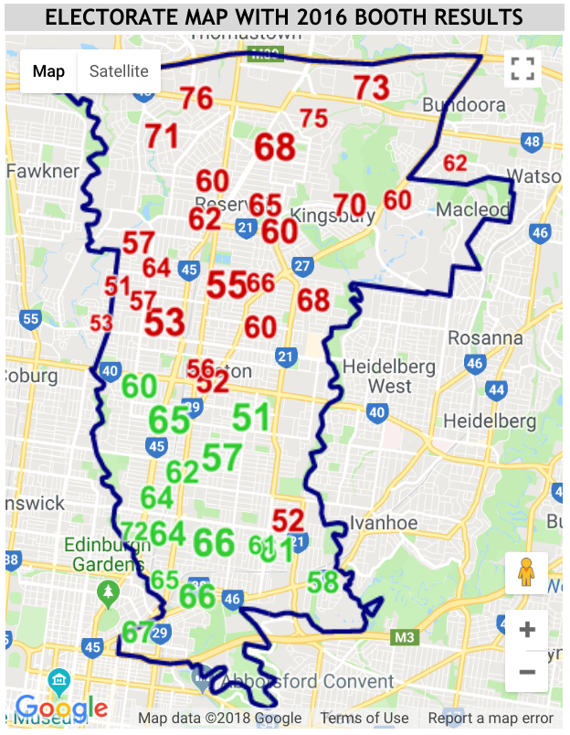
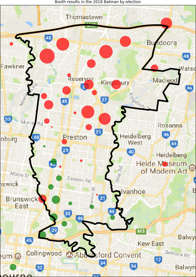