Four point parabolas
Introduction
It is (or should be) well known that a parabola has the cartesian form
\[ (Ax+By)^2+Cx+Dy+E = 0. \]
This looks as though there are five values needed, but we can divide through in such a way as to make any of the coefficients we like equal to 1:
\[ (Px+Qy)^2+Rx+Sy+1 = 0. \]
and so we see that only four values are needed to define a parabola. A parabola thus has one more degree of freedom than a circle, for which only three values are needed:
\[ (x-A)^2+(y-B)^2 = C^2. \]
For any four points "in general position" in the plane, there will be two parabolas that pass through those points. The purpose here is to explore how that can be done.
There are some explanations at mathpages and also here but the confusion of algebra and the old-fashioned typesetting makes these articles hard to read.
It's easiest to do it by an example first, then discuss the general method afterwords.
One way - a bit more complicated than necessary
Suppose we start with four points
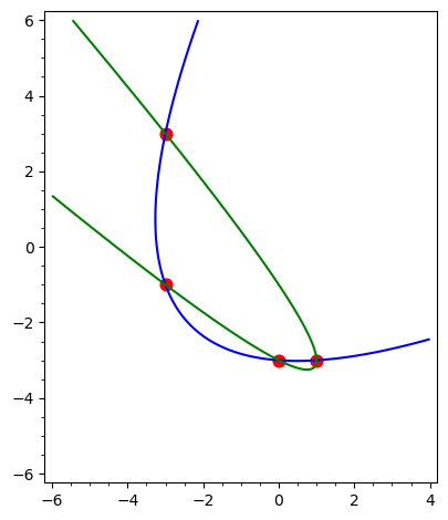
\[ (0,-3),\quad (-3,3),\quad (1,-3),\quad (-3,-1) \]
By substituting each of these values into the first equation above, we obtain four equations:
\begin{gather} (-3B)^2 + 3D + E = 0\\ (-3A+3B)^2-3C+3D+E=0\\ (A-3B)^2+C-3D+E=0\\ (-3A-B)^2-3C-D-E=0 \end{gather}
The plan of attack is this:
- Solve the first three equations for \(C\), \(D\) and \(E\). The results will be expressions in \(A\) and \(B\).
- Substitute the results from step 1 into the last equation, and solve for \(A\) and \(B\). There will in general be two solutions.
- Substitute the newly found values of \(A\) and \(B\) into the expressions for \(C\) and \(D\) to obtain the parabola equations.
And of course we can do all of this in Sage. Here's step 1:
var('A,B,C,D,E,x,y')
xs,ys = [0,-3,1,-3],[-3,3,-3,-1]
eqns = [(A*x+B*y)^2+C*x+D*y+E for x,y in zip(xs,ys)]
sols1 = solve(eqns[:-1],[C,D,E],solution_dict=True)
sols1
This produces:
\[ \left[\left\{C : -A^{2} + 6 \, A B, D : -2 \, A^{2} + 6 \, A B, E : -6 \, A^{2} + 18 \, A B - 9 \, B^{2}\right\}\right] \]
Now for step 2:
sols2 = solve(eqns[-1].subs(sols1[0]),[A,B], solution_dict=True)
This produces:
\[ \left[\left\{A : r_{1}, B : -r_{1}\right\}, \left\{A : r_{2}, B : r_{2}\right\}\right] \]
Note that the parameters in which \(A\) and \(B\) are given may well depend on how many such computations you've done. Sage will simple keep increasing the parameter index each time parameters are needed. (When I performed this particular calculation, the indices were in fact 925 and 926.) You can however re-set the indices by prefixing the above command as follows:
maxima_calculus.reset()
sols2 = solve(eqns[-1].subs(sols1[0]),[A,B], solution_dict=True)
Before we substitute back into the expressions for \(C\), \(D\), \(E\), we turn the parameters into variables:
p = sols2[0][A].free_variables()[0]
q = sols2[1][A].free_variables()[0]
Now for step 3:
s0 = sols2[0]
s1 = sols2[1]
para0 = (s0[A]*x+s0[B]*y)^2+sols1[C].subs(s0)*x+sols1[D].subs(s0)*y+sols1[E].subs(s0)
parab0 = (para0.factor()/p^2).numerator().expand()
para1 = (s1[A]*x+s1[B]*y)^2+sols1[C].subs(s1)*x+sols1[D].subs(s1)*y+sols1[E].subs(s1)
parab1 = (para1.factor()/q^2).numerator().expand()
At this point, the equations of the two parabolas are
\[ x^{2} - 2 x y + y^{2} - 7 x - 8 y - 33 = 0,\qquad x^{2} + 2 x y + y^{2} + 5 x + 4 y + 3 = 0 \]
or, to conform with the general equation from above:
\[ (x-y)^2-7x-8y-33=0,\quad (x+y)^2+5x+4y+3=0. \]
They can be displayed, along with the initial points, like this:
b = 3
xmin,xmax = min(xs)-b,max(xs)+b
ymin,ymax = min(ys)-b,max(ys)+b
p1 = implicit_plot(parab0,(x,xmin,xmax),(y,ymin,ymax))
p2 = implicit_plot(parab1,(x,xmin,xmax),(y,ymin,ymax),color='green')
p3 = list_plot([(s,t) for s,t in zip(xs,ys)],plotjoined=False,marker="o",size=60,color='red',faceted=True)
p1+p2+p3
A slightly simpler way
Shift the points so that one of them is at the origin. For example, with the points above, we could shift by \((0,3)\) to obtain
\[ (0,0),\quad (-3,6),\quad (1,0),\quad (-3,2) \]
Since the parabolas must pass through the origin, we must have \(E=0\), so that we are looking for expressions of the form
\[ (Ax+By)^2+Cx+Dy=0 \]
and we only need to use the three points away from the origin. Then we work very similarly to above, except that we will only use three points and three equations.
a,b = xs[0],ys[0]
xs,ys = [x-a for x in xs[1:]],[y-b for y in ys[1:]]
eqns = [(A*x+B*y)^2+C*x+D*y+E for x,y in zip(xs,ys)]
sols1 = solve(eqns[:-1],[C,D,E],solution_dict=True)[0]
sols1
The outcome of all this is
\[ \left\{C : -A^{2}, D : -2 \, A^{2} + 6 \, A B - 6 \, B^{2}\right\} \]
Now we can substitute and solve for \(A\) and \(B\) as above:
maxima_calculus.reset()
sols2 = solve(eqns[-1].subs(sols1),[A,B], solution_dict=True)
Continuing as before:
p = sols2[0][A].free_variables()[0]
q = sols2[1][A].free_variables()[0]
s0 = sols2[0]
s1 = sols2[1]
para0 = (s0[A]*x+s0[B]*y)^2+sols1[C].subs(s0)*x+sols1[D].subs(s0)*y
parab0 = (para0.factor()/p^2).numerator().expand()
para1 = (s1[A]*x+s1[B]*y)^2+sols1[C].subs(s1)*x+sols1[D].subs(s1)*y
parab1 = (para1.factor()/q^2).numerator().expand()
The two parabolas here are
\[ x^{2} - 2 x y + y^{2} - x - 14y ,\quad x^{2} + 2 x y + y^{2} - x - 2 y \]
To get back to the parabolas we want, simply shift back:
parab0.subs({x:x-a,y:y-b}).expand()
parab1.subs({x:x-a,y:y-b}).expand()
Another example
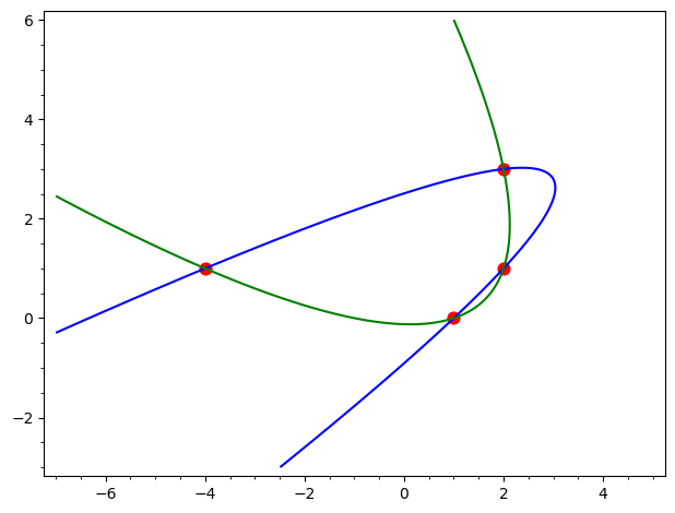
\[ (x,y) = (2,3),\quad (2,1),\quad (-4,1),\quad (1,0). \]
Repeat the above commands with the points shifted to include the origin:
xs0, ys0 = [2,2,-4,1], [3,1,1,0]
a,b = xs0[0],ys0[0]
xs,ys = [x-a for x in xs0[1:]],[y-b for y in ys0[1:]]
eqns = [(A*x+B*y)^2+C*x+D*y+E for x,y in zip(xs,ys)]
sols1 = solve(eqns[:-1],[C,D,E],solution_dict=True)[0]
Now substitute into the last equation and solve for \(A\) and \(B\):
sols2 = solve(eqns[-1].subs(sols1),[A,B], solution_dict=True)
Finally, substitute both equations back to obtain \(C\) and \(D\), and factor out the parameter:
p = sols2[0][A].free_variables()[0]
q = sols2[1][A].free_variables()[0]
s0 = sols2[0]
s1 = sols2[1]
para0 = (s0[A]*x+s0[B]*y)^2+sols1[C].subs(s0)*x+sols1[D].subs(s0)*y
parab0 = (para0.factor()/p^2).numerator().expand()
para1 = (s1[A]*x+s1[B]*y)^2+sols1[C].subs(s1)*x+sols1[D].subs(s1)*y
parab1 = (para1.factor()/q^2).numerator().expand()
We could obtain the same result a bit more easily by letting the variables
p and q be in a tuple, similarly for s0 and s1, and for the parabolas.
This would cut the commands down to four instead of eight.
Before plotting, we need to substitute back in the original \(x\) and \(y\) values by another shift:
parab0 = parab0.subs({x:x-a,y:y-b}).expand()
parab1 = parab1.subs({x:x-a,y:y-b}).expand()
Now plot them; we need to refer to the original xs0, ys0 values:
b = 3
xmin,xmax = min(xs0)-b,max(xs0)+b
ymin,ymax = min(ys0)-b,max(ys0)+b
p1 = implicit_plot(parab0,(x,xmin,xmax),(y,ymin,ymax))
p2 = implicit_plot(parab1,(x,xmin,xmax),(y,ymin,ymax),color='green')
p3 = list_plot([(s,t) for s,t in zip(xs0,ys0)],plotjoined=False,marker="o",size=60,color='red',faceted=True)
p1+p2+p3